SciML & UQ Group

Research

Fast, scalable, and parallel computational methods for learning, prediction, and decisions under high-dimensional uncertainty.

On the computational side, a digital twin needs four things: a fast model, data to correct it, decisions to make, and the computing to run it. Our flood digital twin is where the four come together. The physical side, installing sensors in the field and acting on the real system, is where we collaborate with others.

FlagshipWhere the four come together

Digital twins for real-time flood prediction

Basin-wide flood forecasts in seconds instead of an hour, driven by rainfall, terrain, and a handful of stream gauges.
72 hours of Hurricane Helene (September 2024) simulated with GeoSWE on three nested domains: MRMS rainfall in purple, flood depth in color, and the NOAA CO-OPS tide gauges that drive the coastal boundary as stars. The application runs are computational demonstrations under stated, uncalibrated settings, not validated flood hindcasts.
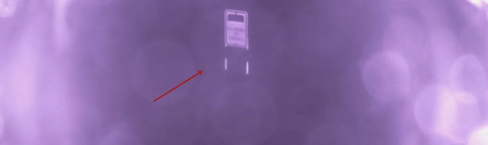
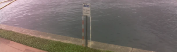
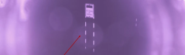
Three views from one camera of a sign and two banded staffs at a seawall: by day, on an ordinary night with four bright bands on each staff, and during Hurricane Helene with a single band left on each
One of the cameras that our collaborators at the University of South Florida have installed in Pinellas County, at the university's waterfront on Bayboro Harbor in St. Petersburg. It looks at two staffs marked with reflective bands, beside a sign: by day (top), on an ordinary night (middle), and on the night of September 26, 2024, during Hurricane Helene (bottom), when only the top band of each staff was still above the water. Photos: CRIS-HAZARD project, University of South Florida.
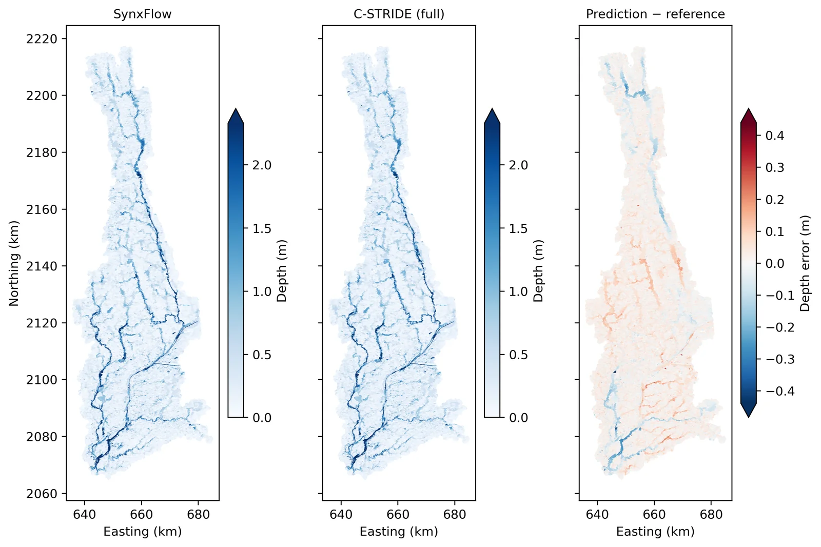
C-STRIDE at work on the April 2013 flood in the Des Plaines River basin. Twelve hours of gauge histories and rainfall are encoded into a latent state; the decoder, guided by coordinates, elevation, slope, and Manning coefficient, turns it into a map of water depth. The prediction follows the SynxFlow simulation through the flood's rise and recession: in the difference, blue marks underprediction and warm colors overprediction. Inference takes about a quarter of a second per field.
Read moreShow less

Emergency managers need to know where floodwater is, how deep it is, and how it will change over the coming hours across an entire river basin. During a flood, however, real-time measurements come from only a handful of stream gauges, and high-resolution hydrodynamic models are too costly to rerun each time new data arrive or to run as large ensembles.

We are building the components of flood digital twins that answer in real time. GeoSWE is a GPU finite-volume solver for the full 2D shallow-water equations, from a 3 m coastal county to the conterminous United States on one multi-GPU node. On the Frontier supercomputer it simulated Hurricanes Helene and Milton across Pinellas County on a 1 m grid with every building, which you can explore in 3D in Two Storms, One Metre. CLDNet, a conditional latent dynamics network surrogate of the shallow water equations, produces a 96-hour basin-wide forecast in about 29 seconds on one GPU, about 115 times faster than the simulator it is trained on. C-STRIDE, an observation-driven AI digital twin, turns short records from a few stream gauges, together with terrain and rainfall, into basin-wide maps of water depth, and extends these predictions up to a day ahead: in the Des Plaines River basin near Chicago, six gauges inform predictions over 4.2 million 30 m grid cells.

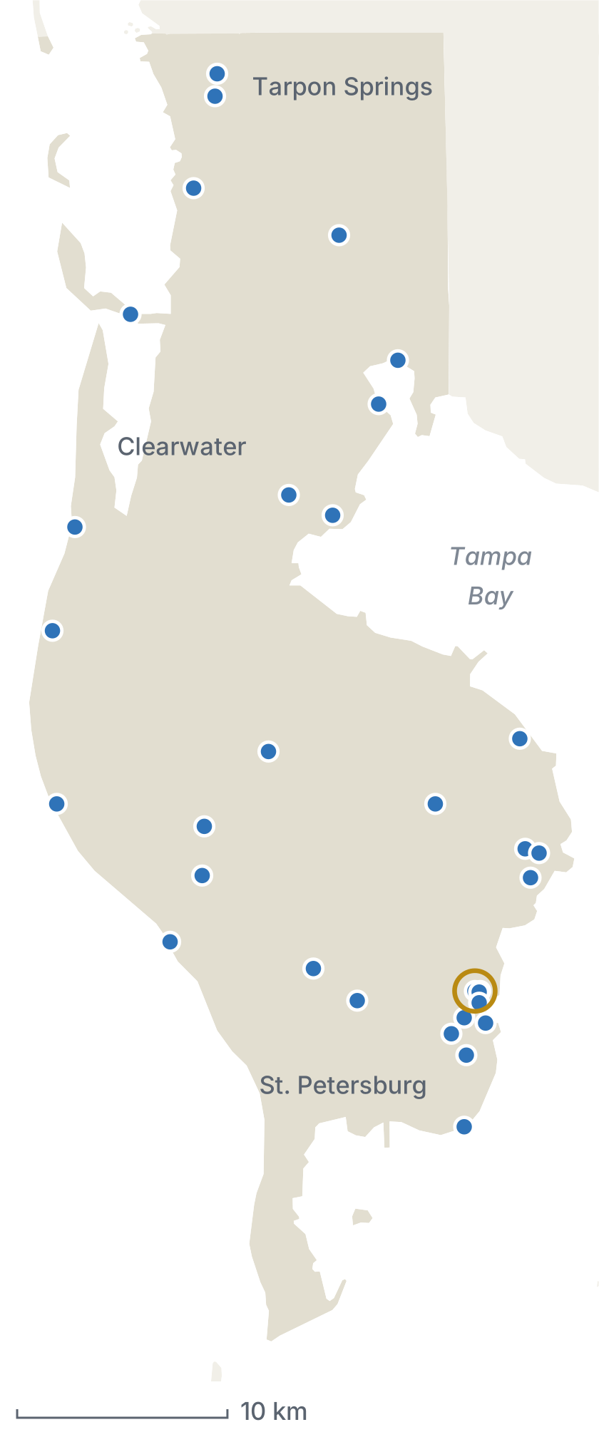
A digital twin also has a physical side: sensors on the real system, and a way for its predictions to reach the people who act on them. In Pinellas County, a low-lying peninsula on Florida's Gulf Coast, our collaborators at the University of South Florida are building this side as CRIS-HAZARD, a community resilience information system led by Prof. Barnali Dixon and funded by the National Science Foundation (award 2325631). They have installed 32 cameras on the coast, along creeks and canals, and inland, aimed at staffs marked with reflective bands so that the water level can be read from the pictures by day and by night, and residents add their own flood reports. Our part is computational: to combine these sparse observations, along with tide gauges, stream gauges, and weather stations, with real-time flood prediction, and to quantify how far the result can be trusted before it goes back to residents and emergency managers.

6 more figures
Water depth in Pinellas County, Florida, during Hurricane Helene: the reference simulation (left), the prediction from ten sensors, marked by crosses (middle), and their difference (right).
Map of Pinellas County, a peninsula between the Gulf and Tampa Bay, with 32 dots on its coasts, creeks and lakes, nearly half of them in St. Petersburg in the south
The 32 cameras of CRIS-HAZARD in Pinellas County, Florida, as listed on the project's public map in October 2026. The ringed camera is the one in the photographs. Land and water: U.S. Census Bureau.
Three maps of the Des Plaines River basin: water depth from the hydrodynamic model, water depth from C-STRIDE, and their difference
C-STRIDE prediction of the April 2013 flood in the Des Plaines River basin at peak total reference depth: depth from the SynxFlow hydrodynamic model (left), from C-STRIDE (center), and prediction minus reference (right).
CLDNet against the reference simulation over 96 hours of a flood in the Des Plaines River basin: the reference water depth across the basin (center), and the depth at eight locations, chosen for the largest peak depth (left) and the largest variation in time (right). Solid lines are the reference, dashed lines the CLDNet forecast.
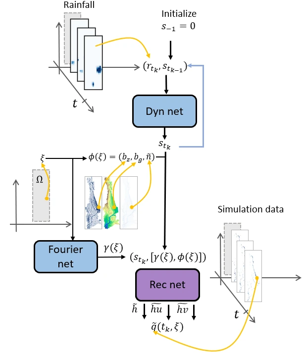
Architecture of CLDNet
CLDNet. Rainfall and the previous latent state drive the dynamics network (Dyn net); the reconstruction network (Rec net) decodes the latent state together with a Fourier embedding of the query coordinate and terrain features into water depth and unit discharges.
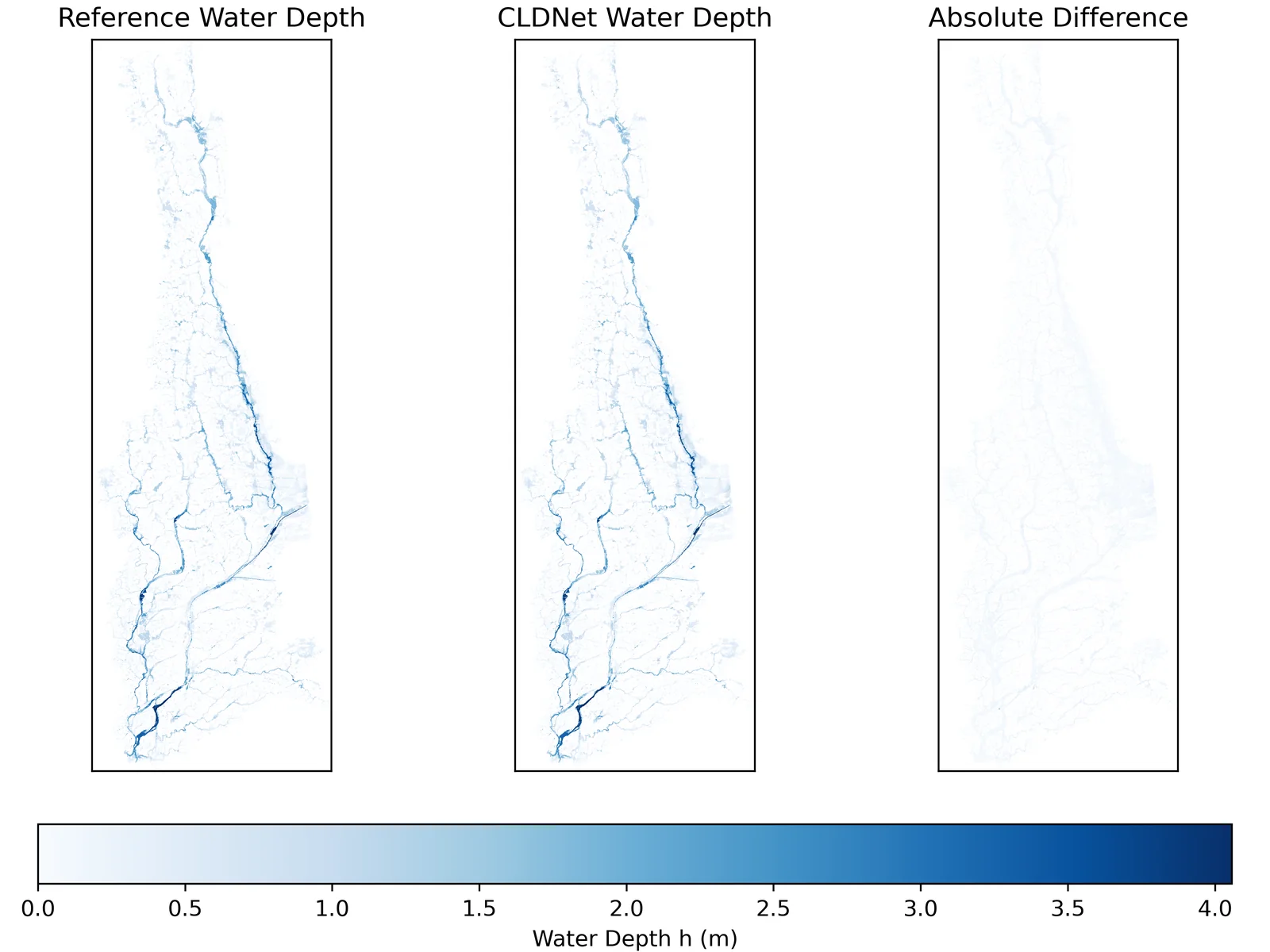
Three maps of the Des Plaines River basin: reference water depth, CLDNet water depth, and their absolute difference
Peak water-depth maps of the Des Plaines River basin for the April 2013 flood, the event for which the reference simulator is validated against USGS gauges: SynxFlow reference (left), CLDNet prediction (center), and absolute error (right).

Selected papers

ModelA fast model of the physics

Operator learning with derivatives and error guarantees

Neural surrogates of PDE solution operators that learn from few simulations, get the derivatives right, and come with error bounds.

Network diagram: an encoder, three residual blocks acting on a few reduced coordinates, and a decoder
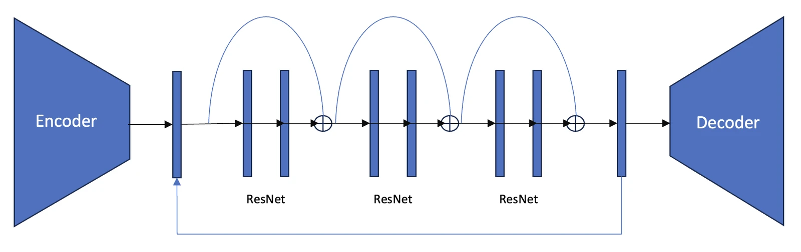
Reduced basis architecture of a derivative-informed neural operator (DINO): an encoder and a decoder given by reduced bases of the input and output functions, with a residual network between the reduced coordinates.
Basis functions of the active subspace and of the Karhunen–Loève expansion
Basis of active subspace (AS) vs Karhunen–Loève expansion (KLE).
Read moreShow less

Bayesian inversion, optimal experimental design, and optimization under uncertainty are outer-loop tasks that solve a PDE again and again. A neural operator that replaces the solver has to be trained from a limited number of expensive simulations, and because these tasks rely on the derivatives of the solution map, it has to approximate the derivatives as well as the values.

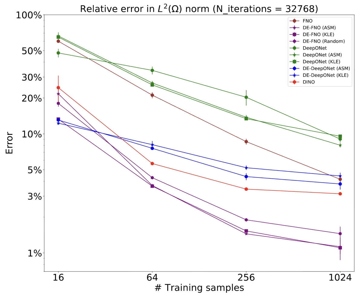
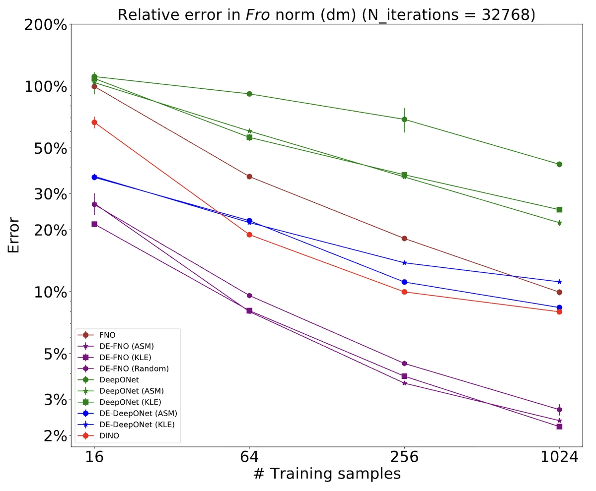
Derivative-informed projected neural networks (DIPNet) project the high-dimensional input and output functions onto derivative-informed low-dimensional subspaces and train a parsimonious network whose size is independent of the discretization. Derivative-informed neural operators (DINO) add the derivatives to the training loss at a cost comparable to training without them, and DE-DeepONet carries the idea to DeepONet and Fourier neural operators. Both are more accurate than operators trained on function values alone, for the solution and for its derivatives, especially when training data are limited.

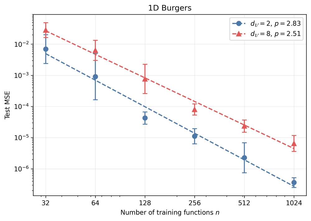
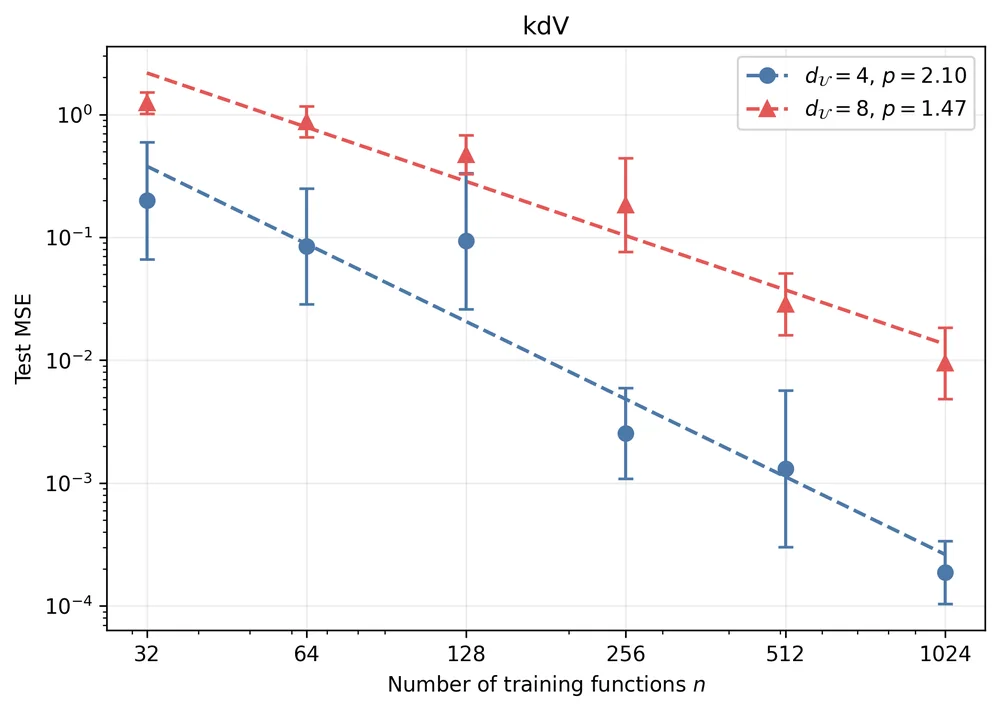
We also ask when such surrogates can be trusted. Our analysis of reduced basis neural operators bounds the approximation errors of the operator and of its derivatives, from the dimension reduction, the network, and the sampling. The variationally correct reduced basis neural operator is trained on a first-order system least-squares residual that is provably equivalent to the solution error, so the loss itself is a computable a posteriori error estimator. For transformer operator networks, we establish a power scaling law between the prediction error and the number of training samples, with an exponent that reflects the intrinsic dimension of the input functions.

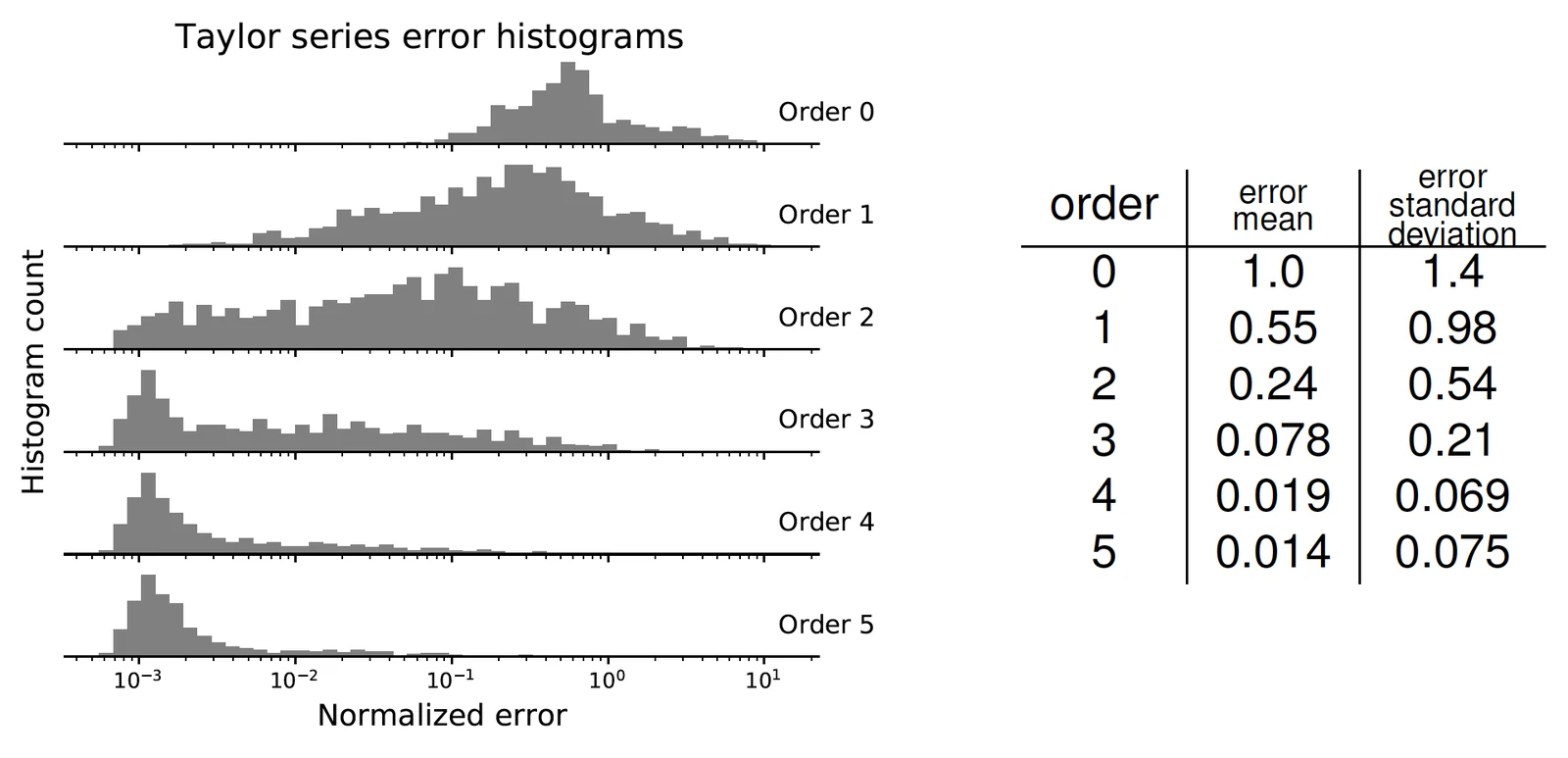
The Tucker tensor train Taylor series (T4S) is a local alternative to global operator learning: a high-order Taylor surrogate fitted from derivative probes at a single expansion point, with each derivative tensor represented as a Tucker tensor train. Earlier, we developed a scalable randomized algorithm for converting tensors into tensor train format based on actions of the tensor as a multilinear map, which allows efficient compression of large high-order derivative tensors for nonlinear mappings that are implicitly defined through the solution of a system of equations.

5 more figures
Two charts of relative error against the number of training samples for ten neural operators; the derivative-enhanced ones lie below their counterparts
Training with derivatives on a hyperelasticity problem: relative error of the solution (lefttop) and of its derivative with respect to the input parameter (rightbottom) against the number of training samples. Each derivative-enhanced operator (DE-FNO, DE-DeepONet) is more accurate than its counterpart trained on solution values alone, for the solution and for the derivative.
A sample of the input field and of the velocity of a turbulent jet, and two charts of eigenvalue decay for the input and output subspaces
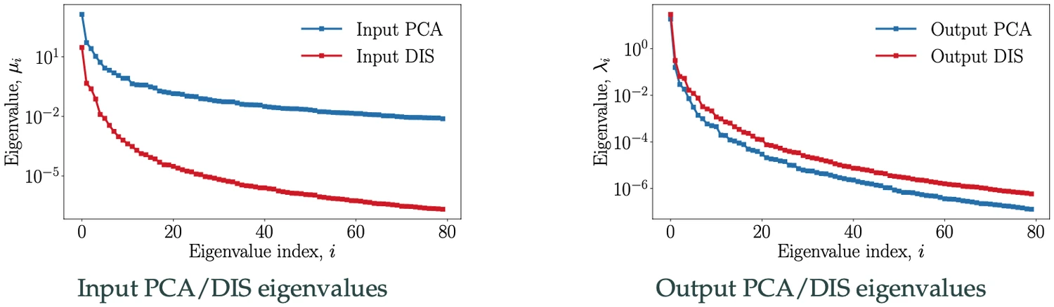
Dimension reduction for a turbulent jet flow: a sample of the uncertain input and of the velocity (top), and the eigenvalues of the input and output subspaces computed by principal component analysis (PCA) and from derivatives (DIS) (bottom). For the input, the derivative-informed eigenvalues decay several orders of magnitude faster.
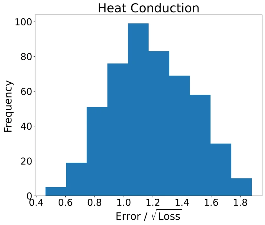
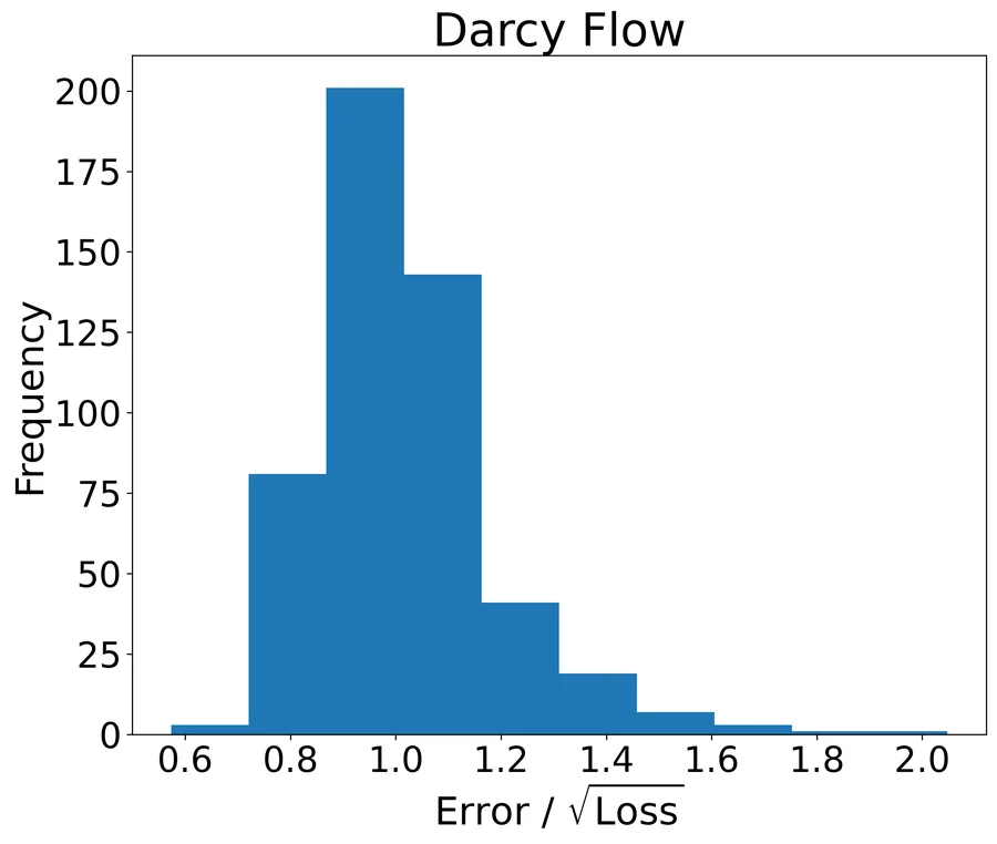
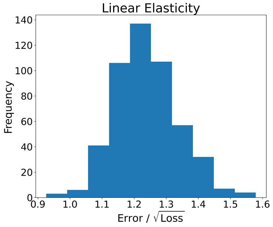
Three histograms of the ratio of error to the square root of the loss, each concentrated around one
The loss as an error estimator. Histograms of the ratio between the error of the reduced basis neural operator and the square root of its residual loss over 500 test samples, for heat conduction, Darcy flow, and linear elasticity.
Test error against the number of training functions on logarithmic axes, with fitted straight lines, for the Burgers and KdV equations
Empirical data scaling of a transformer operator network for the Burgers (lefttop) and KdV (rightbottom) equations: test error against the number of training functions n, for two intrinsic dimensions dU of the input functions. Dashed lines show the fitted power law MSE ≈ C n−p.
Histograms of Taylor series errors for orders 0 to 5, with a table of mean errors
Convergence of functional Taylor approximation by tensor decomposition.

Selected papers

5 more papers

UpdateData to correct it

Data assimilation in latent space

Keeping forecasts of high-dimensional, chaotic systems on track with sparse and noisy observations.

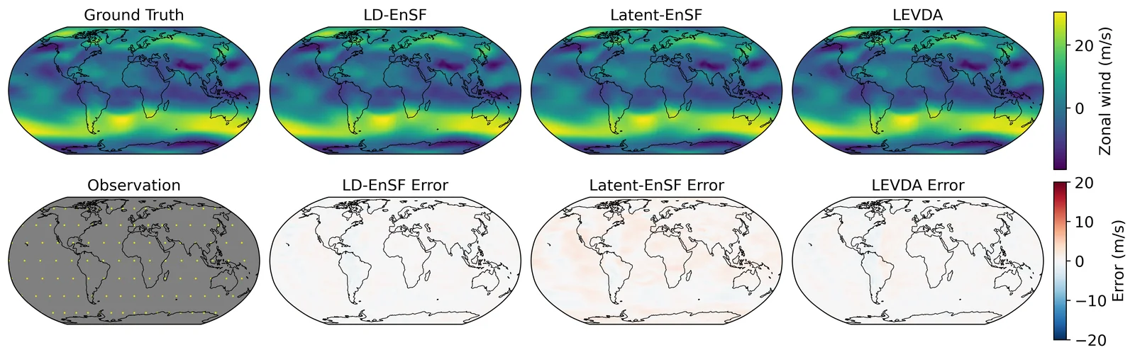
World maps of zonal wind: the ground truth and sparse observations, and the states assimilated by LD-EnSF, Latent-EnSF and LEVDA with their errors
Atmospheric benchmark: zonal wind at 500 hPa at the final assimilation time. The ground truth and its sparse observations (left) are compared with the states assimilated by LD-EnSF, Latent-EnSF, and LEVDA, and their errors.
Read moreShow less

Accurate prediction of complex physical systems relies on data assimilation to correct the errors of model simulations with observations. Traditional ensemble Kalman filters and the more recent ensemble score filters face significant challenges when the states are high-dimensional, the dynamics are nonlinear, and the observations are sparse, which is the usual situation in practice.

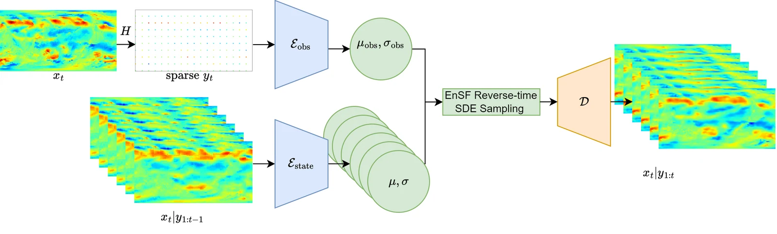
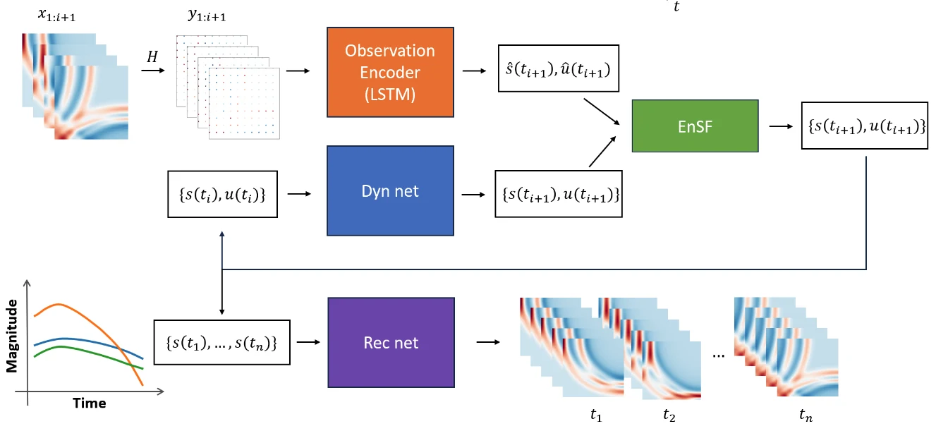
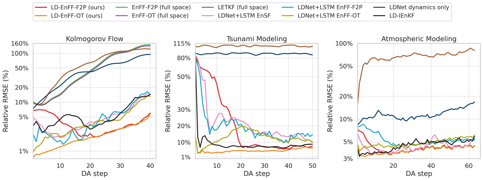
We move the assimilation into a learned low-dimensional latent space. Latent-EnSF encodes the full states and the sparse observations consistently with a coupled variational autoencoder and runs an ensemble score filter there. LD-EnSF also evolves the dynamics in the latent space, with latent dynamics networks and an LSTM encoder of the observation history, which eliminates the full-space simulations and gives speedups of orders of magnitude. LEVDA is the variational counterpart: a four-dimensional ensemble-variational smoother in the latent space of a differentiable neural dynamics surrogate, which assimilates states and unknown parameters jointly, without adjoint code, from observations at arbitrary locations and times. LD-EnFF replaces the score filter with an ensemble update based on flow matching and evaluates the observation likelihood in latent space. The benchmarks include Kolmogorov flow, tsunami propagation, and atmospheric dynamics, with noisy observations that are sparse in both space and time.

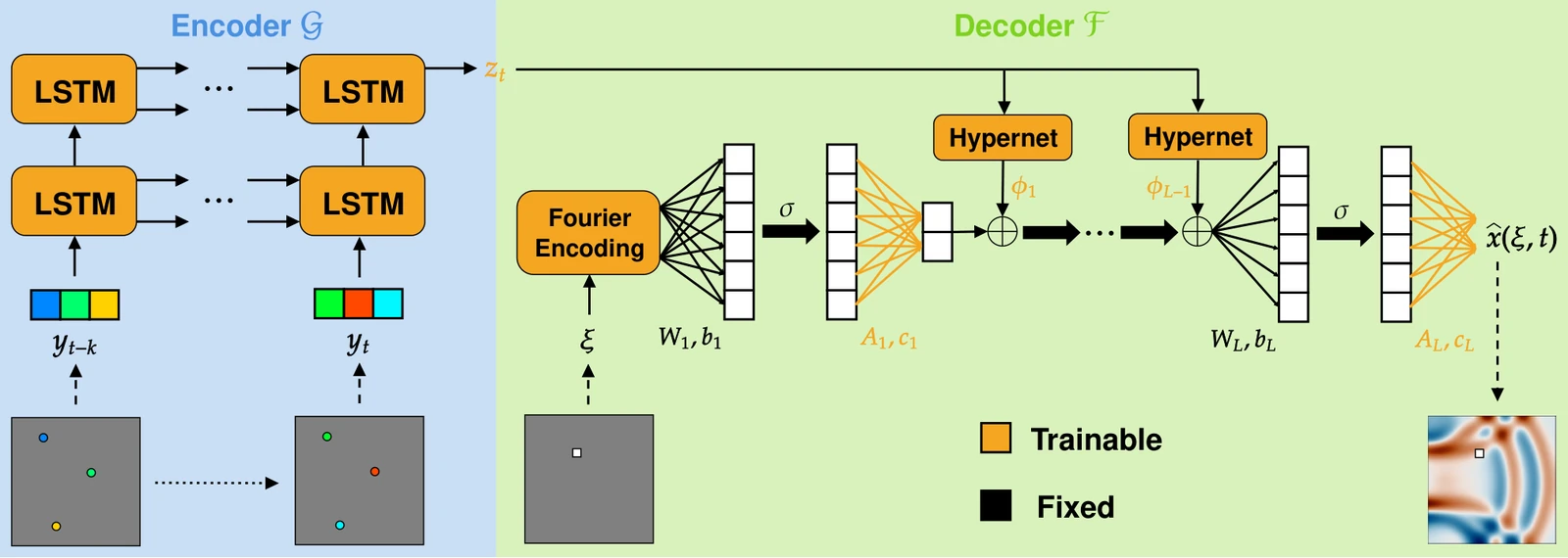
A related question is how much of a field can be recovered from a few point sensors alone. STRIDE maps a short window of sensor measurements to a latent state with a temporal encoder and reconstructs the field at arbitrary locations with an implicit neural decoder. C-STRIDE in our flood digital twin extends it with terrain and rainfall.

8 more figures
Diagram of the Latent-EnSF pipeline: encoders for the state and the sparse observation, score-filter sampling in latent space, and a decoder
Flow of the Latent-EnSF. An ensemble of prior states xt | y1:t−1 is assimilated with sparse observation yt in the latent autoencoder space to obtain samples xt | y1:t from the posterior.
Diagram of the LD-EnSF pipeline
Flow of the LD-EnSF. An ensemble of historical sparse observations y1:i+1 is mapped (by LSTM) and assimilated (by EnSF) to the latent dynamics and decoded to the full dynamics.
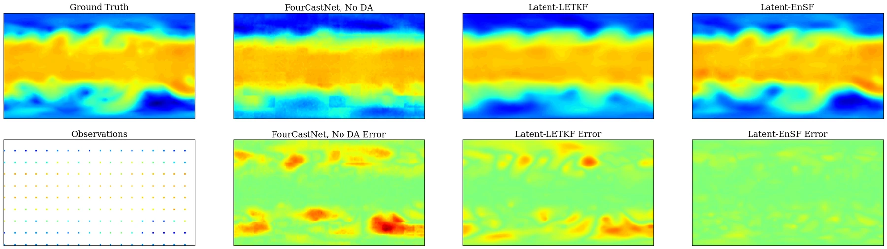
Maps of 500 hPa geopotential from reanalysis and from three forecasts, with the sparse observations and the forecast errors
Medium-range weather forecasting on ERA5 reanalysis with the FourCastNet model: geopotential at 500 hPa after 41 days, assimilating once a day observations that are 64 times sparser than the state. Top: ground truth, FourCastNet without data assimilation, Latent-LETKF, and Latent-EnSF. Bottom: the observations and the errors of the three forecasts.
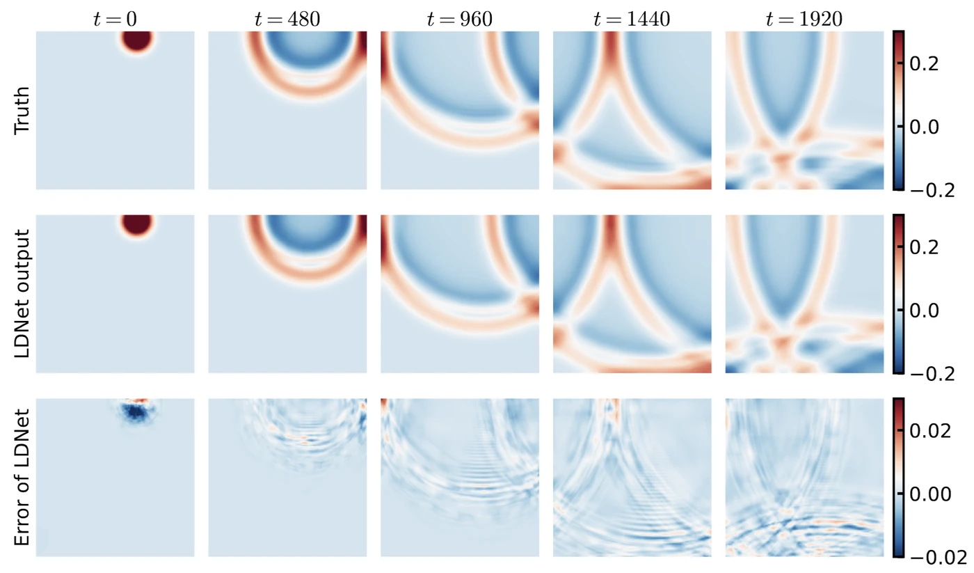
A wave spreading across a square basin at five times: reference, network output, and the much smaller error
A latent dynamics network on the tsunami benchmark: the reference solution (top), the network output (middle), and its error (bottom) at five times. The error is about 2%.
Two of the benchmark systems: shallow water wave propagation (left) and Kolmogorov flow (right).
Three charts of relative error against assimilation step for ten data assimilation methods
Mean relative RMSE of the full state over 20 held-out test trajectories for Kolmogorov flow, tsunami modeling, and atmospheric modeling: LD-EnFF against latent-space and full-space baselines.
Diagram of STRIDE: a recurrent encoder of the sensor history, and a decoder network evaluated at a query location
STRIDE. A temporal encoder maps the sensor history yt−k:t to a latent variable zt, and a modulated implicit neural representation decodes it into the field at arbitrary locations ξ.
STRIDE on a shallow water benchmark, over a test trajectory: the ground truth and the observations at 100 random locations used as input (first column), followed by the predictions and errors of STRIDE and of baseline models.

Selected papers

2 more papers

Bayesian inference in high dimensions

Learning models from data, with their uncertainty, when the unknown is a field with thousands to millions of parameters.

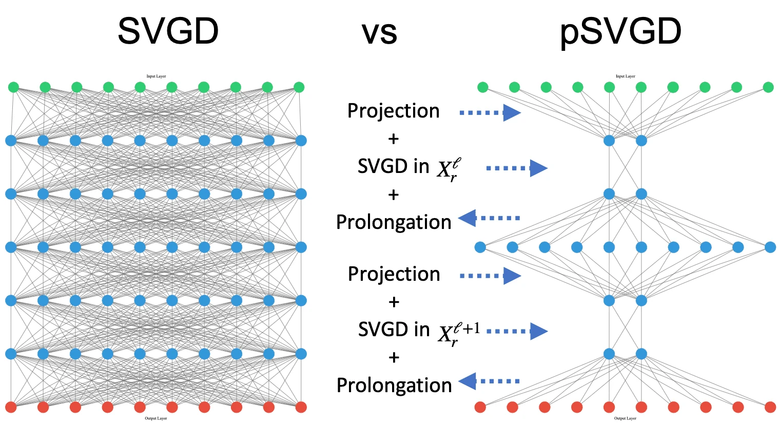
SVGD compared with pSVGD, which alternates projection, SVGD in a subspace, and prolongation
Project high-dimensional parameters to data-informed low-dimensional subspaces that are adaptively constructed using the gradient or Hessian of the parameter-to-observable map at current samples.
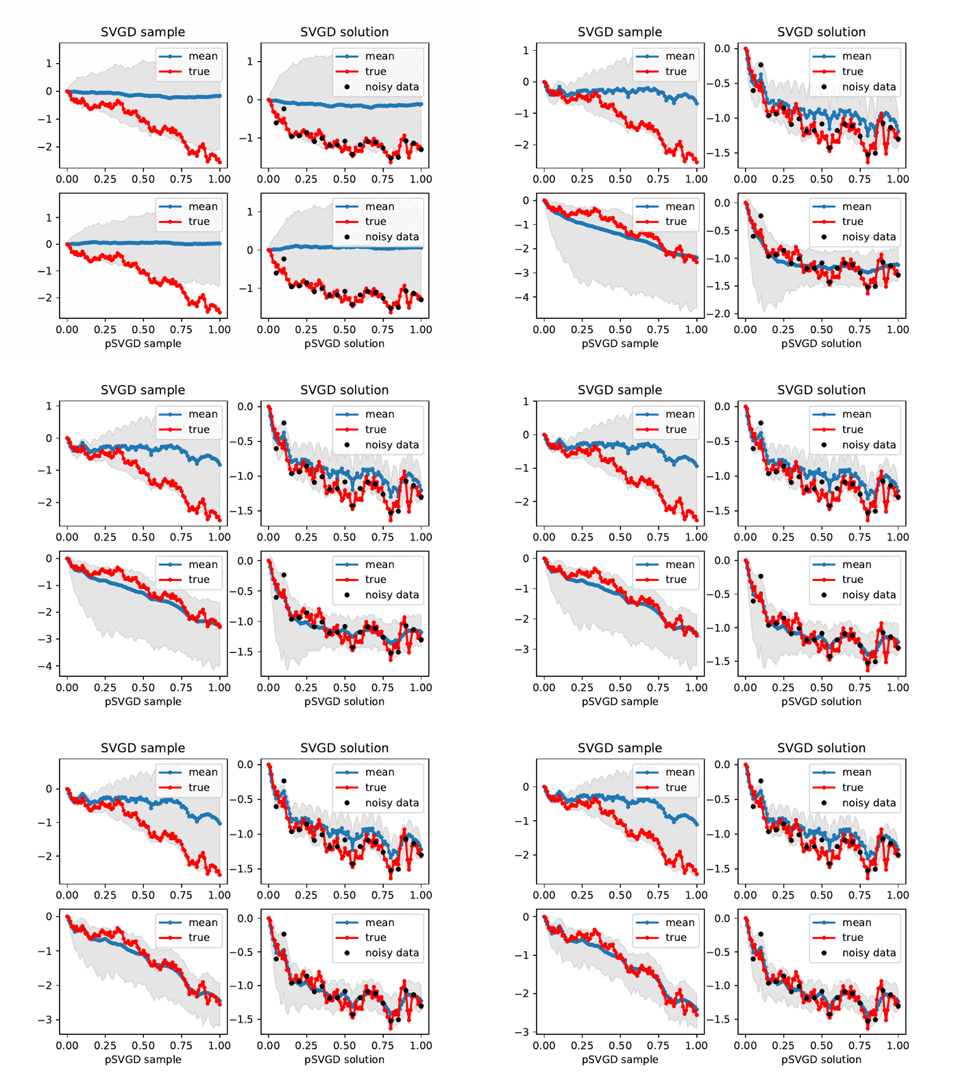
Animation of SVGD and pSVGD samples converging over iterations
Evolution of SVGD (top) and pSVGD (bottom) parameter samples and their corresponding solutions of a conditional-diffusion model at iteration l = 0, 10, ..., 100. Shown are the true, sample mean, 90% credible interval, and noisy data.
Read moreShow less

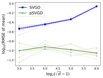
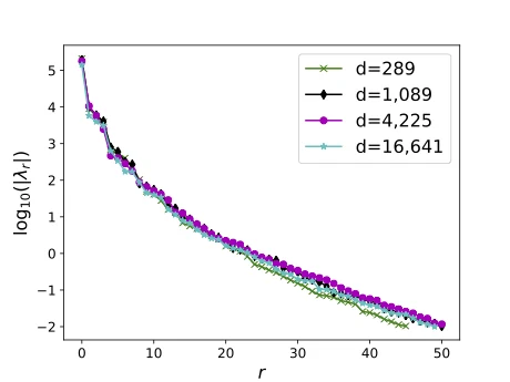
By exploiting the intrinsic low-dimensional geometric structure of the posterior distributions in high-dimensional Bayesian inverse problems, we developed projected variational inference methods (pSVGD and pSVN) to tackle the curse of dimensionality faced in such problems. The methods are demonstrated to be fast, accurate, and scalable with respect to the number of parameters, samples, data points, and parallel processor cores for scientific, engineering, and machine learning problems.

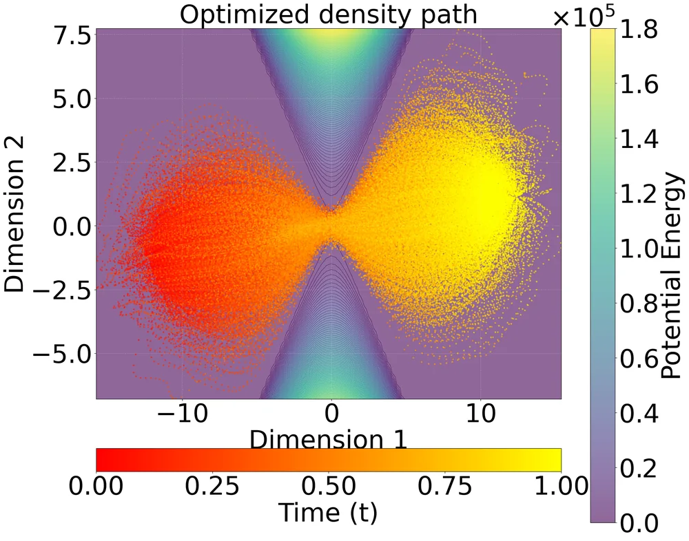
We also work with other transports of probability distributions. Projected Wasserstein gradient descent (pWGD) projects the parameters into a low-dimensional subspace to overcome the curse of dimensionality of kernel density estimation, and a convex semidefinite program gives the optimal approximation of the Wasserstein gradient direction in a class of two-layer neural networks. PDPO computes action-minimizing paths between probability densities by representing the path as the pushforward of a reference density through a parametric map; three to five control points of a spline in parameter space suffice for multimodal and high-dimensional problems.

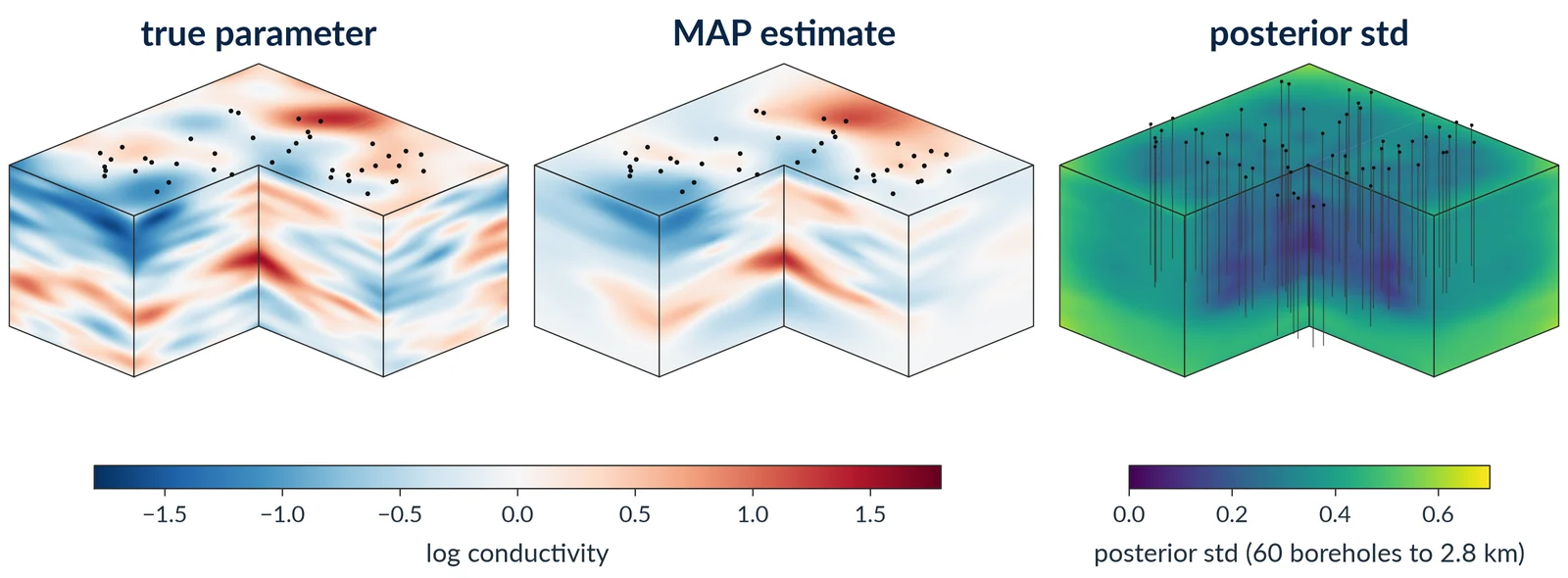
For Bayesian inverse problems governed by PDEs at scale, hIPPyMFEM provides the full workflow on GPUs, from the MAP point and a low-rank Laplace approximation of the posterior to MCMC. In a geothermal application it solves the forward problem with 1.08 billion state unknowns on 30 GPUs, and infers the conductivity of the rock on a 1283 mesh from temperatures logged in 60 boreholes.

5 more figures
Geothermal application with hIPPyMFEM. Left, heat flowing through the rock of a reservoir: a forward solve at 1.08 billion state unknowns (5123) on 30 GPUs. Right, the conductivity of the rock inferred on a 1283 mesh from temperatures logged in 60 boreholes: the MAP estimate, samples of the posterior, and its standard deviation, lowest where the boreholes reach.
A cloud of particles moving from left to right through the narrow neck between two obstacles, colored by time
A density path optimized by PDPO through the neck of an obstacle potential. Time runs from red (t = 0) to yellow (t = 1).
Sample error against parameter dimension, and eigenvalue decay
pSVGD preserves sample accuracy in increasing parameter dimension d (left) by exploiting the intrinsic low-dimensionality r detected by eigenvalues (right).
Eigenvalues for different numbers of data points, and time against processor cores
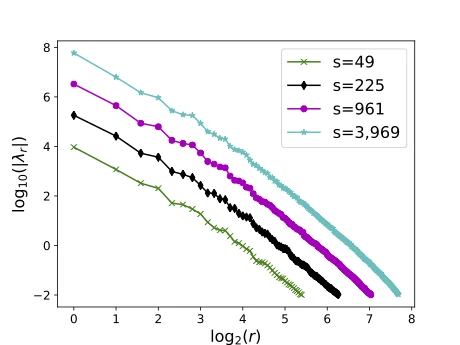
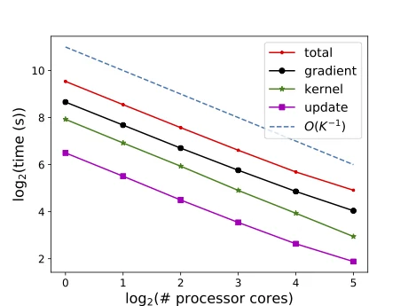
Weak scalable in # data (left) and strong scalable in # processor cores (right).
Samples on a double-banana shaped posterior from three methods, and a chart of the distance to the reference samples over the iterations
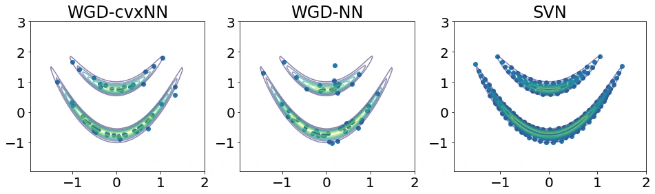
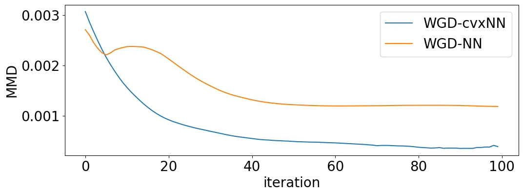
Samples of a double-banana posterior after 100 iterations of Wasserstein gradient descent, with the gradient direction approximated by a two-layer network through a convex program (WGD-cvxNN) or by training (WGD-NN), beside reference samples from the Stein variational Newton method (SVN). RightBottom: the maximum mean discrepancy to the reference samples at each iteration.

Selected papers

2 more papers

DecideDecisions to make

Bayesian optimal experimental design

Where, when, and what to measure, so that each experiment tells us as much as possible.

Pointwise standard deviation of the parameter field under the prior and under posteriors with uniform, static optimal, and adaptive optimal designs
When to image a growing tumor: pointwise standard deviation of the parameter field under the prior distribution and under the posterior distributions with uniform design, static optimal design, and adaptive optimal design (left to right).
Read moreShow less

Experiments and sensors are expensive, so we would like to choose the most informative ones before any data are collected. Bayesian optimal experimental design does this by maximizing the expected information gain. This involves a double integration over the unknown parameters and the possible data, a Bayesian inverse problem for every candidate design, and, when sensors are selected from a set of candidates, a combinatorial optimization.

We make this tractable for models governed by PDEs with infinite-dimensional parameters. The low-rank structure of the parameter-to-observable map and an offline–online decomposition remove the PDE solves from the design optimization. Derivative-informed neural operators then supply the MAP points and the eigenvalues that the optimality criteria need: for selecting sensors in a three-dimensional nonlinear convection–diffusion–reaction problem with tens of thousands of parameters, the speedup is more than 1000×, counting both offline construction and online evaluation.

When experiments are run in sequence, each design should adapt to the data already seen. A derivative-informed latent attention neural operator (LANO) chooses the times at which to take MRI images to monitor tumor growth, with an amortized speedup of 180×. A design policy trained by policy-gradient reinforcement learning places sensors online to track a contaminant source, about 100× faster than high-fidelity finite element methods, and discovers a strategy of moving the sensors upstream. For MRI data acquisition with binary sampling masks, a conditional normalizing flow is trained jointly with a probabilistic formulation of the design.

5 more figures
Network diagram: encoders of the parameter and of the initial state, latent dynamics stepping through time, and decoders of the state and of its Jacobian
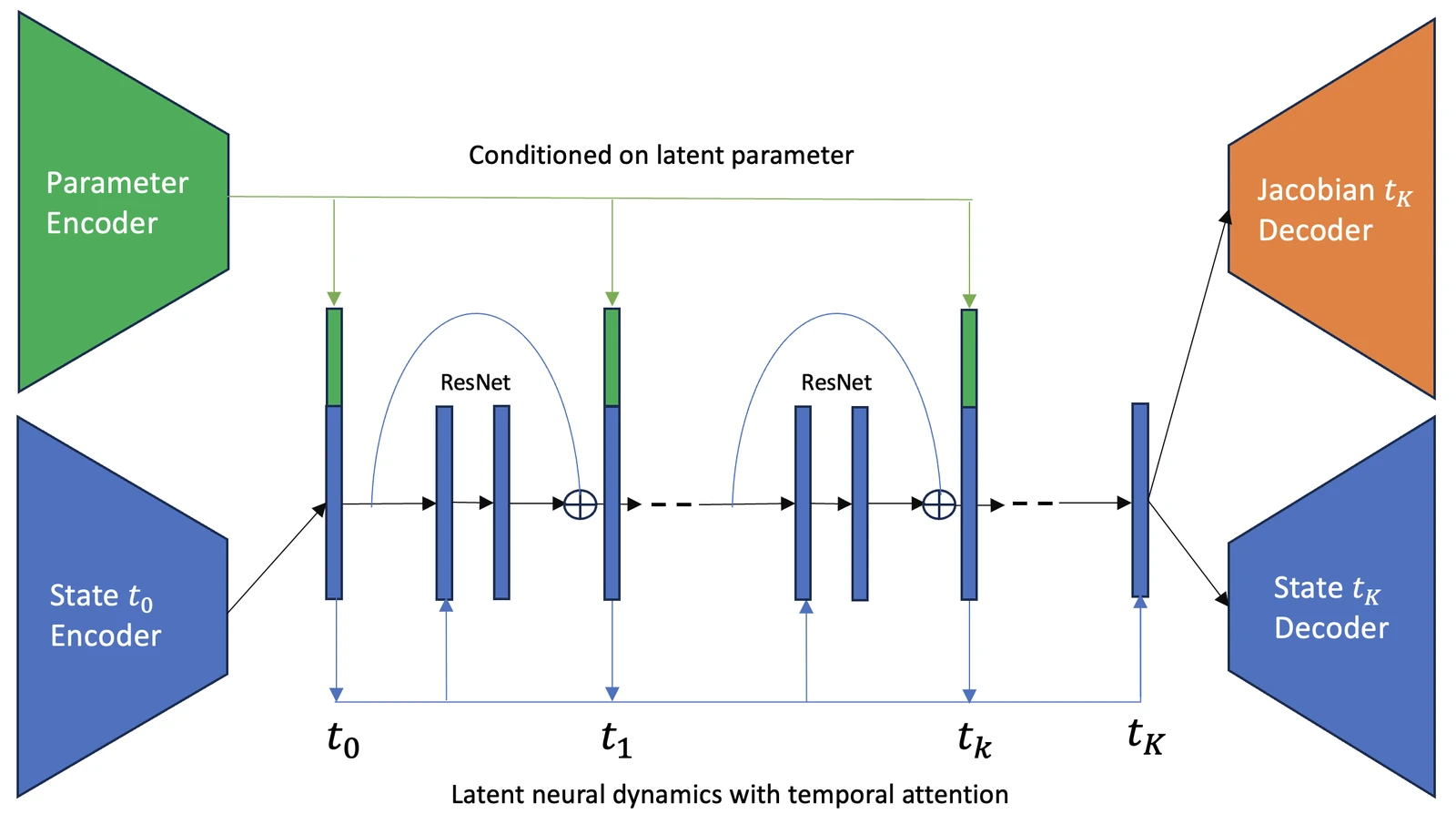
LANO, the derivative-informed latent attention neural operator: the parameter and the initial state are encoded, a latent dynamics with temporal attention advances the state through the observation times, conditioned on the latent parameter, and decoders return the state and its Jacobian.
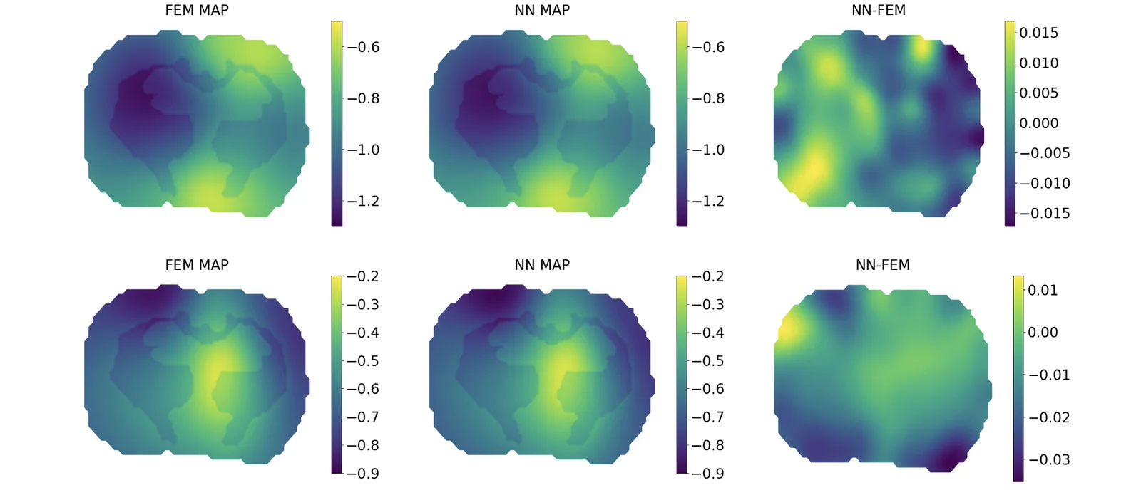
MAP points computed by finite elements and by the neural surrogate, and their difference
MAP points computed by the finite element method (left) and by the LANO surrogate (middle), and their difference (right), for a random sample drawn from the prior. Top: daily observations; bottom: observations at days 2, 5, and 8.
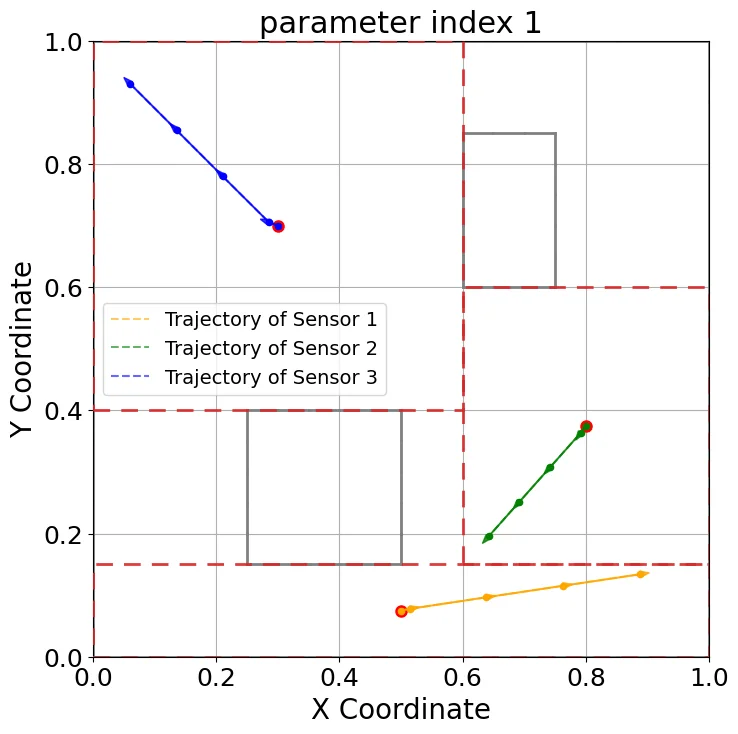
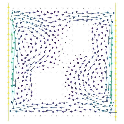
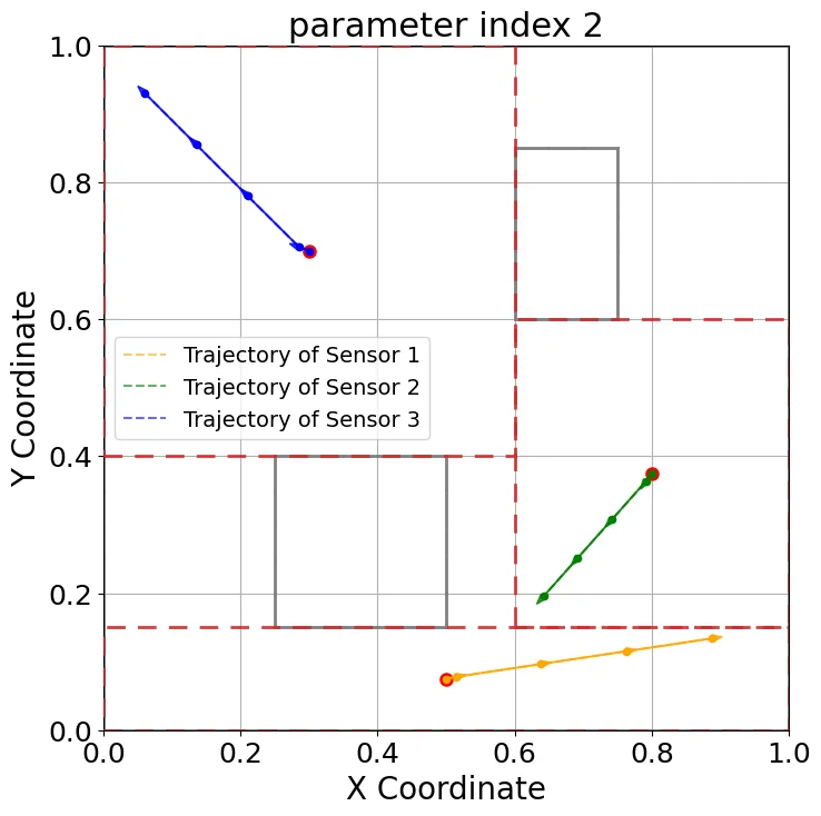
Trajectories of three sensors in their admissible regions for two parameter samples, and the velocity field of the flow
A design policy learned by reinforcement learning for tracking a contaminant source: optimized trajectories of three sensors for two parameter realizations (lefttop and middle). The sensors consistently move upstream against the velocity field (rightbottom) in their admissible domains.
The contaminant concentration around two obstacles over time: finite element solution (left), LANO surrogate (middle), and their difference on the same color scale (right).
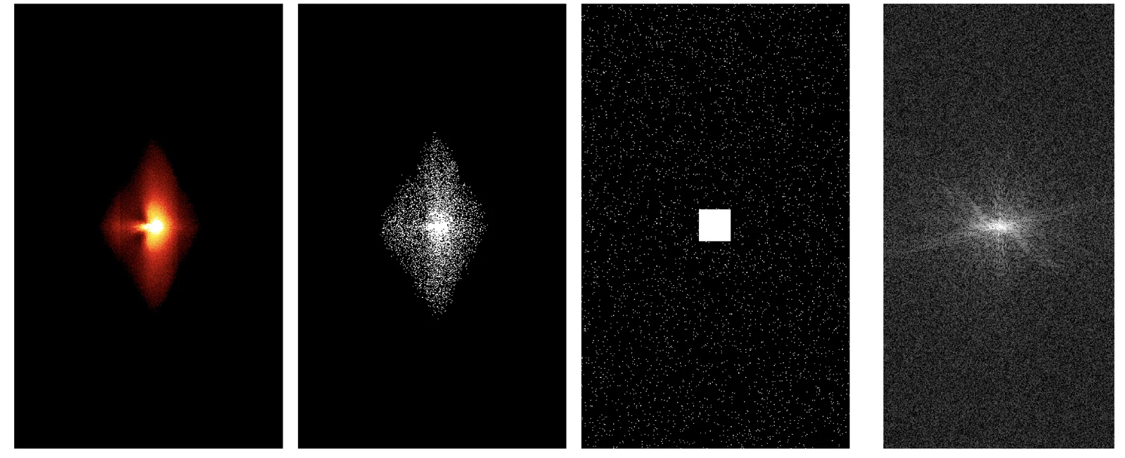
Learned probabilistic and binary MRI sampling designs, a hand-crafted baseline, and fully sampled data
Experimental design for MRI data acquisition with conditional normalizing flows. From left to right: learned probabilistic design, learned binary design, hand-crafted baseline design, and fully sampled data.
5 more papers

Optimization under uncertainty

Designs and controls that still perform when materials, manufacturing, and operating conditions are uncertain.

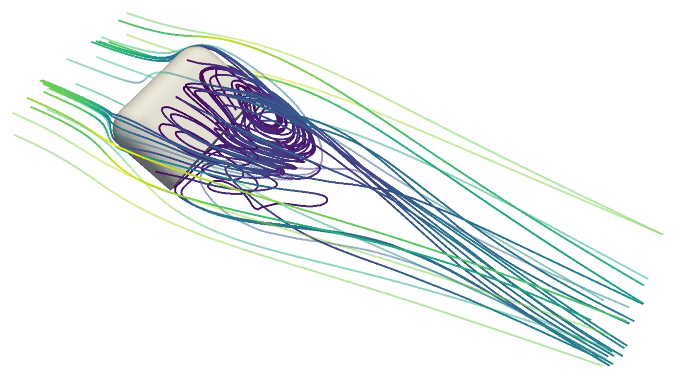
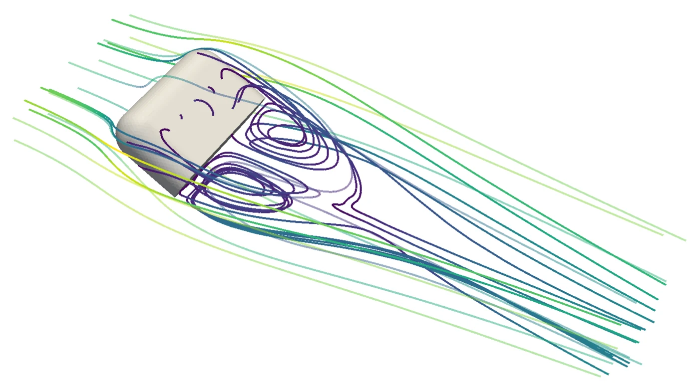
Streamlines of a three-dimensional flow past a bluff body: a large tangled wake without control, a more compact one with control
Risk-averse boundary control of a three-dimensional flow past a bluff body under a random inflow: streamlines of one sample of the flow, uncontrolled (lefttop) and controlled (rightbottom). The flow has over a million unknowns; with MR-DINO trained on 448 samples, the optimization takes 53 seconds.
Read moreShow less

A design that is optimal under nominal conditions can fail once manufacturing errors, uncertain material properties, or a random environment enter. Optimizing a risk measure instead requires a large number of samples at every iteration of the optimization, each one an expensive PDE solve, while the random parameters and the design variables are both high-dimensional.

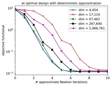
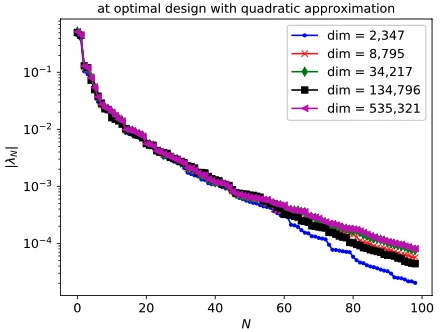
We develop Taylor approximations and neural operators that reduce this cost by orders of magnitude. A Taylor approximation-based approximate Newton method designs an acoustic metamaterial cloak that hides an obstacle under manufacturing errors and incident waves from multiple angles and frequencies; it is scalable, in terms of the number of PDE solves, with respect to both the uncertain parameter dimension (up to half a million) and the optimization variable dimension (over one million). Gaussian mixture Taylor approximations keep the accuracy when the input variances are large, and estimate the conditional value-at-risk to within 1% with on the order of 10 PDE solves, comparable to Monte Carlo with on the order of 10,000 samples. Multi-input reduced basis derivative-informed neural operators (MR-DINO) solve risk-averse control problems for semilinear elliptic and Navier–Stokes equations with random field inputs 103 to 107 times faster in execution, and more than 10 times cheaper once the cost of training is included.

On the theory side, we establish performance bounds for approximation-based algorithms: the optimality gap of the computed controls becomes arbitrarily small as the inaccuracies of discretization, sampling, smoothing, and penalization vanish. Scalable algorithms for PDE-constrained optimization under uncertainty are available in our open-source library SOUPy.

4 more figures
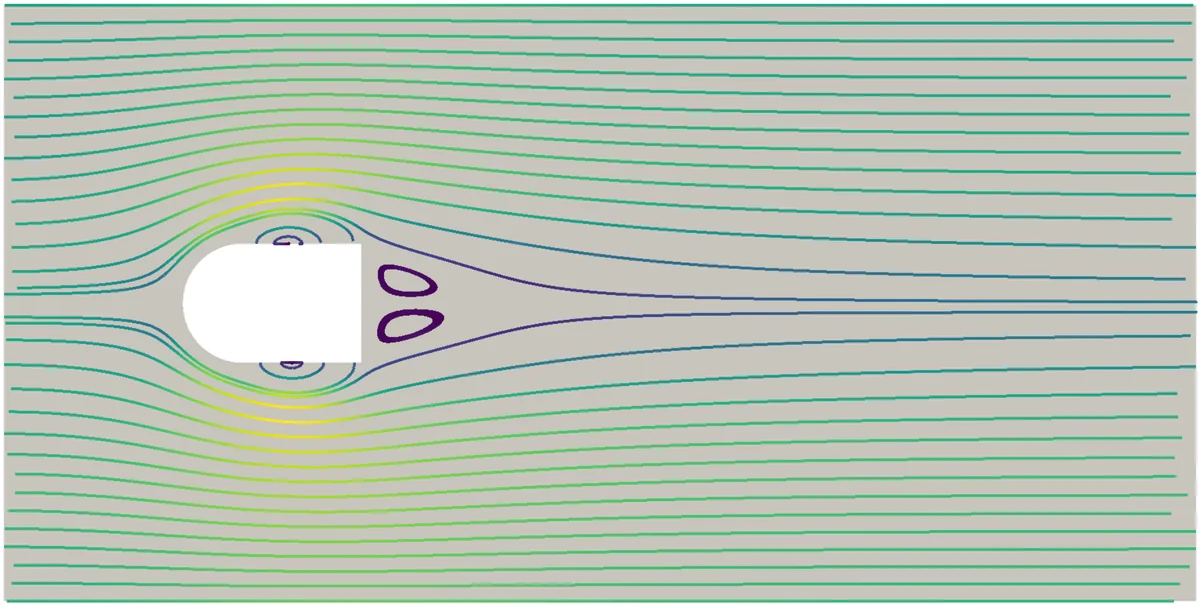
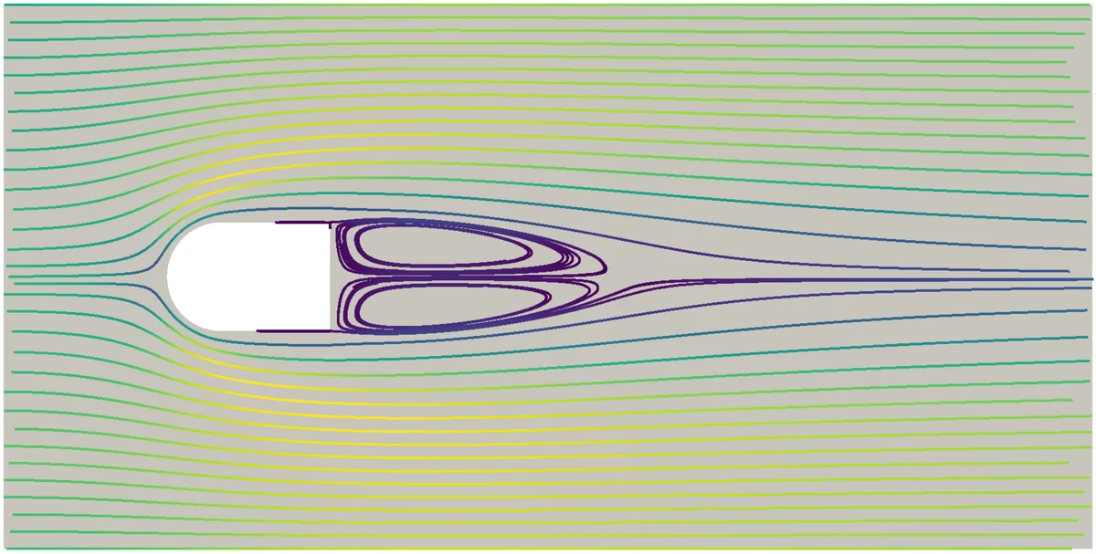
Streamlines of a flow around a bluff body: a long recirculation zone without control, a much smaller one with the optimal control
Risk-averse control of the steady Navier–Stokes equations under uncertainty: a sample of the flow field with no control (lefttop) and with the optimal control (rightbottom), computed using MR-DINO with 256 training samples.
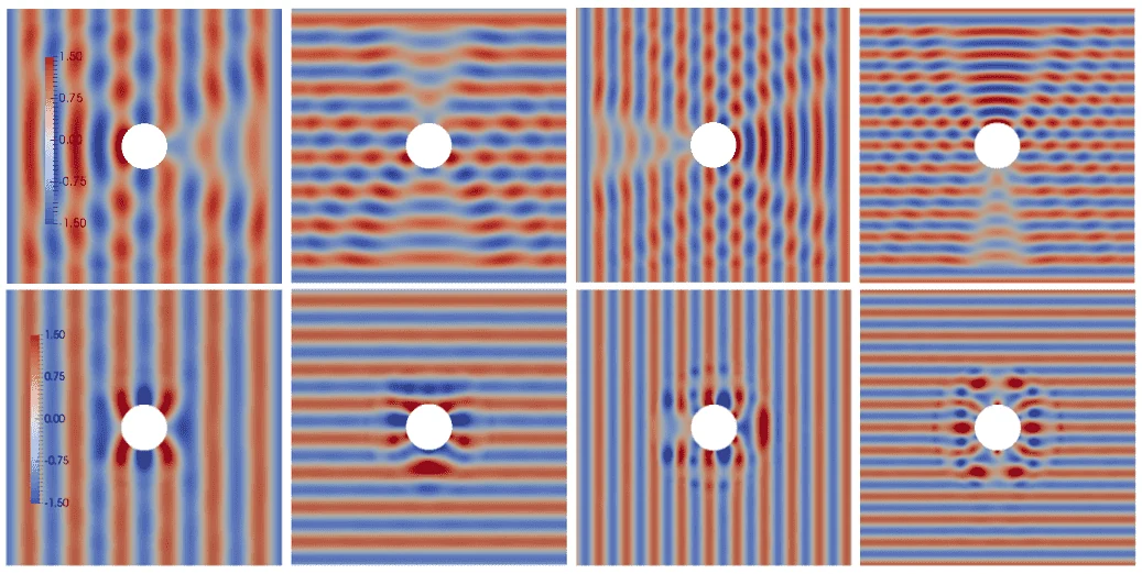
Wave fields around an obstacle without and with a metamaterial cloak
Total wave without (top) and with (bottom) metamaterial cloak around an obstacle, under attack of manufacturing errors, incident waves from multiple angles and frequencies.
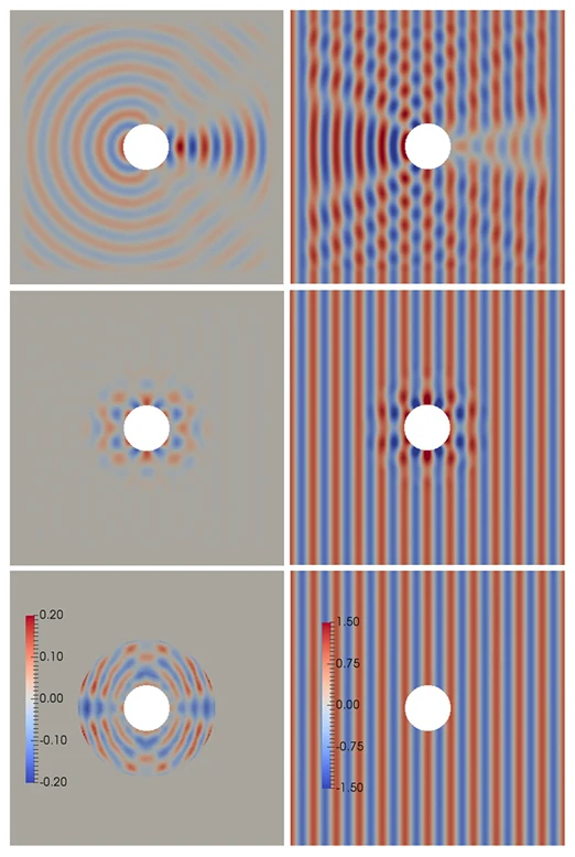
Scattered and total waves around an obstacle, with and without the optimal metamaterial
Top: scattered wave (left) and total wave (right) around an impenetrable obstacle. Middle: scattered wave (left) and total wave (right) with optimal metamaterial present around the obstacle. The scattered wave is eliminated by the metamaterial. Bottom: optimal design (left) and incident wave (right).
Convergence of the optimization, and eigenvalue decay of the Hessian
Convergence of the approximate Newton method (lefttop) and eigenvalues of the Hessian of a parameter-to-output map that represent the intrinsic parameter dimensions.

Selected papers

5 more papers

ScaleThe computing to run it

High-performance computing on GPUs

Simulation and inversion codes written for GPUs, from a single node to the largest machines.

Two charts of time per step against the number of GPUs and of nodes, flat at the ideal line up to 128 nodes
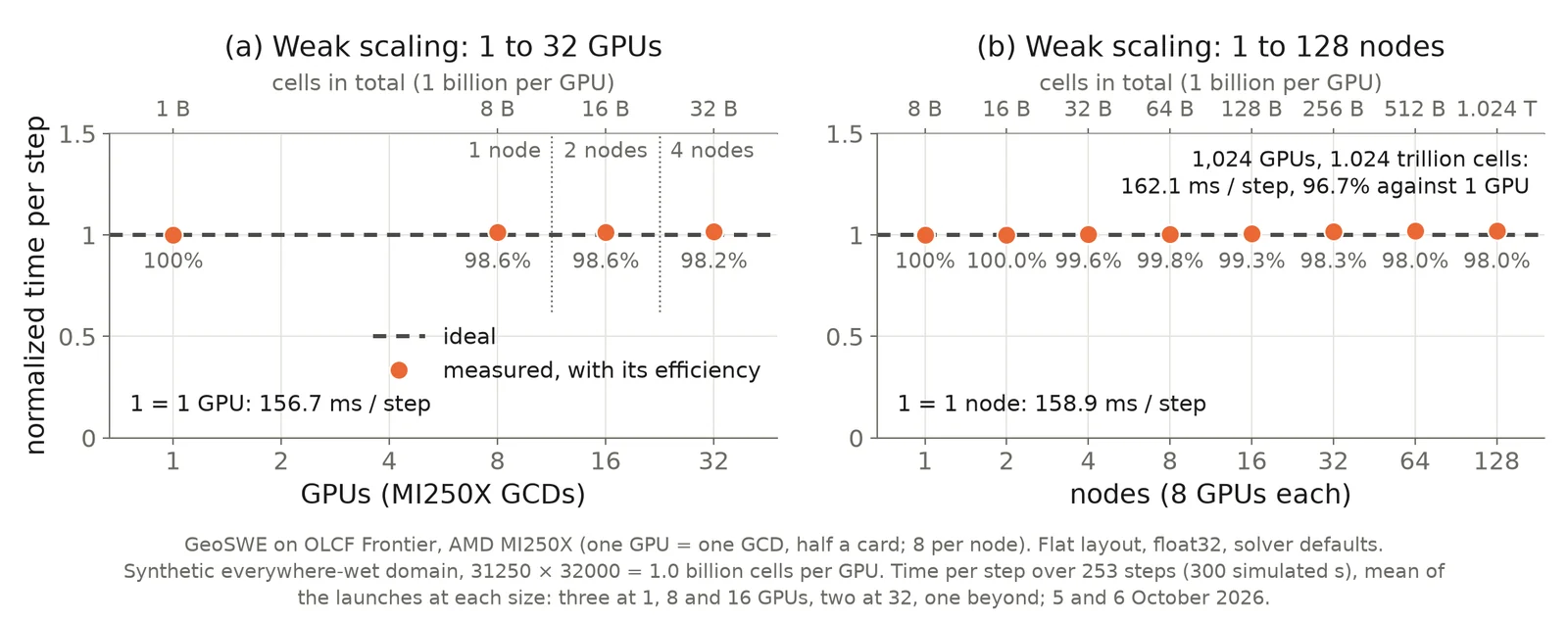
GeoSWE on the AMD GPUs of OLCF Frontier at one billion cells per GPU: time per step divided by that of the smallest size, so ideal weak scaling is the dashed line. On 128 nodes, 1.024 trillion cells advance at 162 ms per step.
Read moreShow less

Digital twins, Bayesian inversion, and the training of surrogates all rest on forward models that are fast at the scale of the real system: a continent at 30 m resolution, or a PDE with a billion unknowns. We write these codes for GPUs and release them as open source.

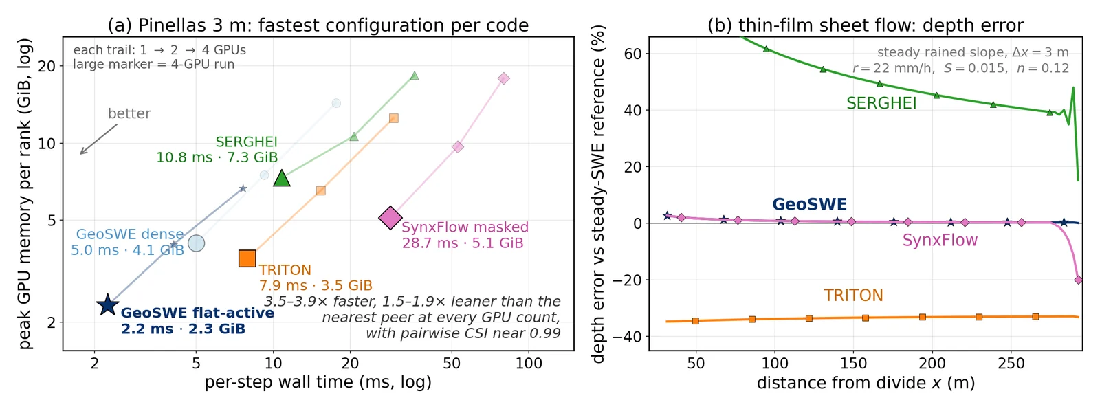
GeoSWE solves the full 2D shallow-water equations on NVIDIA and AMD GPUs. Its compressed active-cell mesh packs the cells that matter into flat arrays, so memory and work scale with the flooded landscape rather than its bounding rectangle. A 72-hour Hurricane Helene scenario over the conterminous United States at 30 m, with 8.88 billion active cells, runs on the eight GPUs of one node in 10.8 hours. On a 214-million-cell county benchmark against TRITON, SynxFlow, and SERGHEI, it has the lowest wall time and GPU memory at every GPU count. On OLCF Frontier, 1.024 trillion cells on 128 nodes advance at 162 ms per step, a weak-scaling efficiency of 96.7% against a single GPU.

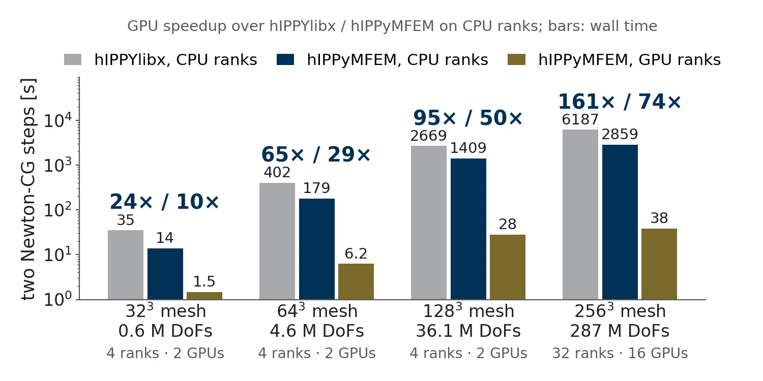
hIPPyMFEM runs Bayesian inverse problems governed by PDEs on GPUs by differentiable programming: the residual, the Jacobian, the adjoint, and every Hessian block come from one JAX function by automatic differentiation, with no derivative coded by hand. Two Newton-CG steps at 287 million unknowns take 38 seconds on 16 GPUs, 161 times faster than hIPPYlibx on 32 CPU cores, and at 1.09 billion unknowns they take 134 seconds on 24 GPUs. The whole Bayesian workflow, from the MAP point and a low-rank Laplace posterior to samples and pointwise variance, takes 10 minutes on four GPUs for a problem with 36 million unknowns.

3 more figures
Wall time against GPU memory for four shallow-water codes, and depth error on a rained slope
(a) Per-step wall time against peak GPU memory per rank for each code's fastest configuration on the 3 m Pinellas County benchmark (1, 2, and 4 GPUs; large marker = 4 GPUs). (b) Depth error against the steady shallow-water reference on a uniformly rained slope.
Bar chart of the time for two Newton-CG steps at four mesh sizes on CPU and GPU ranks
Two Newton-CG steps of a benchmark inverse problem at four mesh sizes: hIPPYlibx and hIPPyMFEM on CPU ranks, and hIPPyMFEM on as many GPU ranks, 24 to 161 times faster than hIPPYlibx.
Three blocks of rock: the true conductivity, its estimate, and the uncertainty left, with the boreholes drawn in
A geothermal inverse problem with hIPPyMFEM: the true log conductivity of the rock, the MAP estimate from temperatures logged in 60 boreholes, and the posterior standard deviation.

More methods and applications

Overview of PolyMicros: generated 3D microstructures, super-resolution of a low-resolution volume, and expansion of a 2D image into 3D

2026

A foundation model for polycrystalline microstructure

Read moreShow less

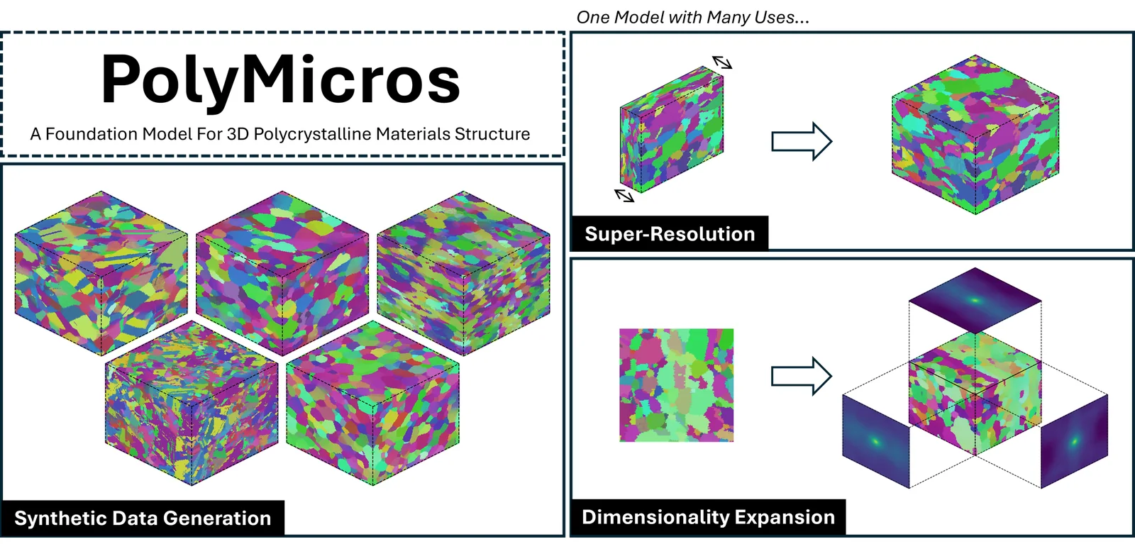
Foundation models for materials have so far been restricted to classes with multi-million sample repositories, while for many structural materials only a few examples exist. With Surya Kalidindi's group, we developed a physics-driven data augmentation scheme, an ensemble of local generative models trained on as few as five experimental observations and coordinated by a diversity curation strategy, to construct PolyMicros, the first foundation model for polycrystalline materials. It solves several long-standing challenges in accelerating 3D experimental microscopy zero-shot.

Corner plot of posterior densities of mass ratio, total mass and effective spin

2024

Bayesian inference in gravitational-wave astronomy

Read moreShow less

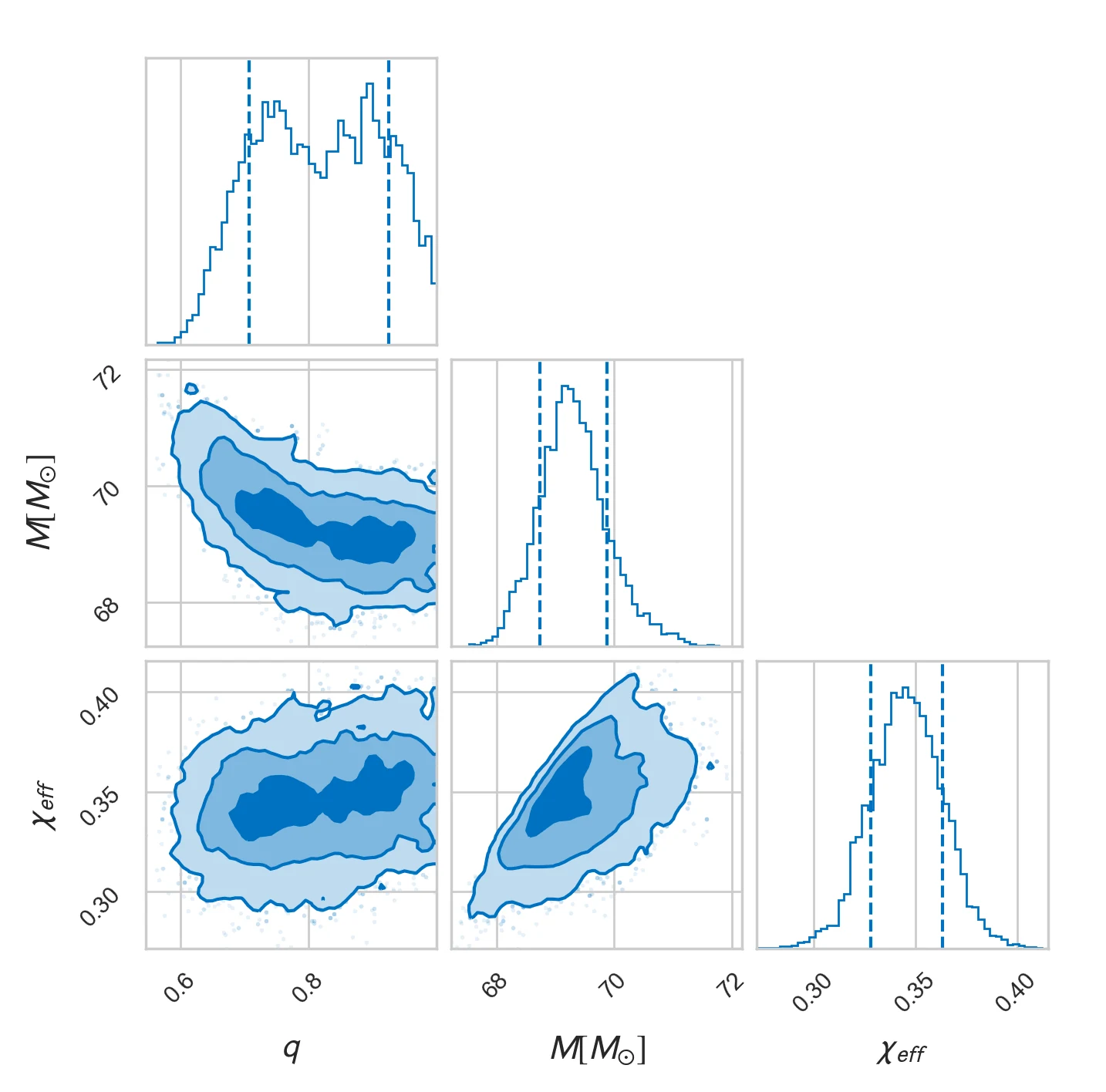
In collaboration with astrophysicists, we develop fast multifidelity Bayesian inference methods to learn the parameters that characterize compact binary systems such as black holes, enabled by a rich hierarchy of surrogates of the numerical relativity that solves Einstein's field equations. Tempered multifidelity importance sampling tempers the biasing distribution of the low-fidelity model for a better overlap with the target posterior, and improves the sampling efficiency on real gravitational-wave detections.

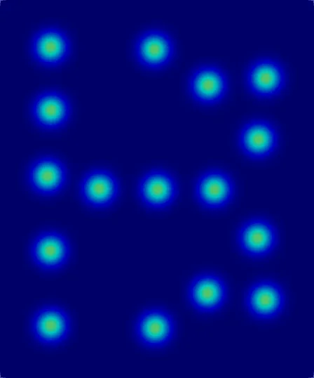
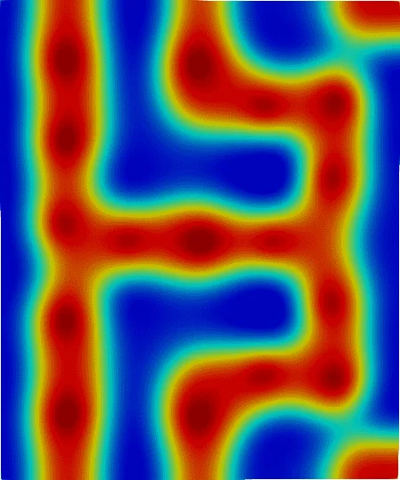
Guiding posts placed by the optimization, and the block copolymer pattern they produce

2023

Directed self-assembly of block copolymers

Read moreShow less

Directed self-assembly of block copolymers is one of the most promising developments in the cost-effective production of nanoscale devices: chemically patterned substrates direct the phase separation into the morphologies needed for semiconductor devices. With a phase field model given by a nonlocal Cahn–Hilliard equation, our inexact Newton algorithm designs the guiding posts of the substrate five orders of magnitude faster than previous work, in two and three dimensions. We also calibrate the model by Bayesian inference from the power spectrum of microscopy images.

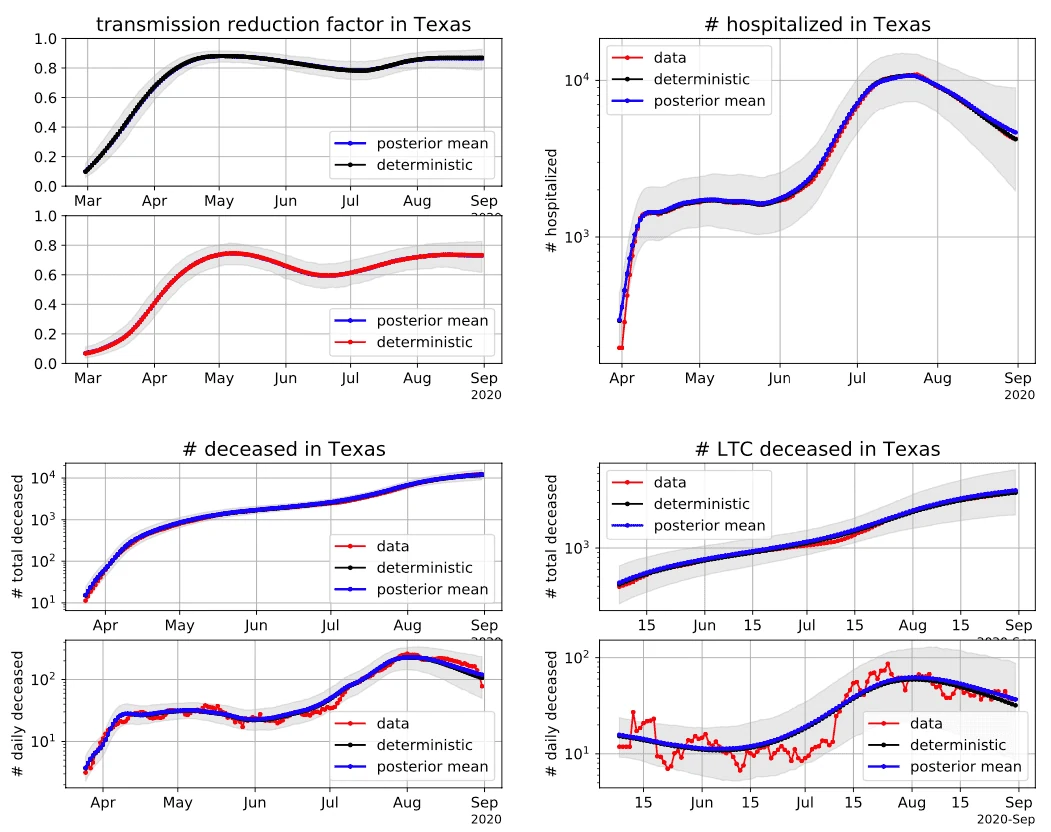
Inferred transmission reduction factor and fits to hospitalized and deceased counts in Texas, with uncertainty

2021

Learning and mitigating COVID-19

Read moreShow less

In the observation of the overwhelming share of COVID-19 deaths from long-term care (LTC) facilities, we developed a data-driven decision-making framework: an LTC-stratified SEIRHD compartment model, Bayesian inference of the model parameters (about 1500 dimensions) using our pSVGD method, and stochastic optimization of the mitigation policy under parameter and operation uncertainties, to reduce deaths and mitigation burden subject to a chance constraint of hospital capacity.

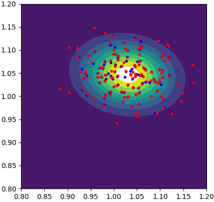
Samples computed with the full and with the reduced model, scattered over the contours of a posterior density

2013–2021

Structure-exploiting model reduction

Read moreShow less

A reduced order model (ROM) compresses a high-fidelity model with certified and computable error bounds while preserving the model structure, which enables many-query statistical learning and stochastic optimization, real-time predictive simulation, and system control. By exploiting the structures of different models, probability distributions, and computational goals, we developed weighted, goal-oriented, localized, adaptive, and learning algorithms for uncertainty quantification, reliability and failure probability analysis, Bayesian inverse problems, optimal control, and optimal experimental design.

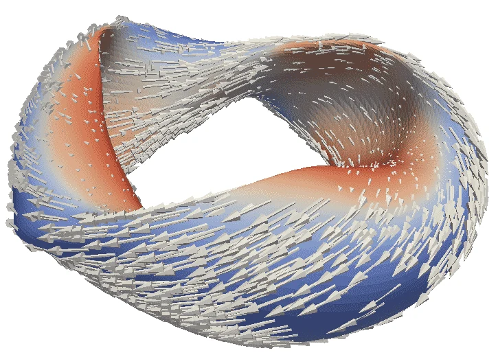
Magnetic field vectors on a twisted toroidal plasma surface

Stellarator design for plasma fusion

Read moreShow less

In the Simons Collaboration, we work on stochastic optimization for the design of the shape of stellarator devices, which facilitate magnetic confinement of plasma fusion in order to harness nuclear fusion power. Quasisymmetry, a concept critical to sustain stable plasma fusion, is optimized subject to manufacturing errors (which led to the termination of the NCSX construction) and operation uncertainties, employing automatic differentiation and parallel GPU computing.

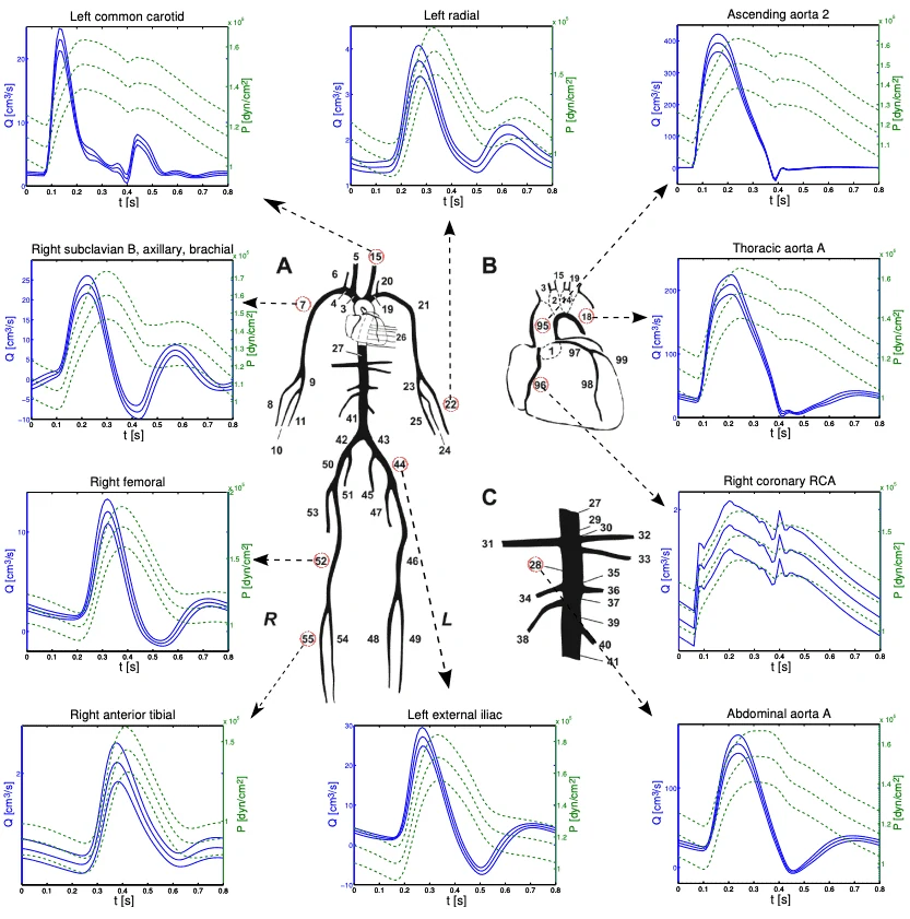
Blood flow rate and pressure with uncertainty in the human arterial network

2013

Uncertainty quantification of human arterial networks

Read moreShow less

We conducted uncertainty quantification and global sensitivity analysis of human arterial networks with 150 physiological parameters. The results help for better understanding of the influence of different physiological abnormalities to various cardiovascular diseases such as heart attack, stroke, aneurysms, aorta stiffening.

The bigger picture

Our broad research interests are in the multidisciplinary fields of computational mathematics, data science, scientific machine learning, and parallel computing with various applications in computational science and engineering (CSE). Specifically, we are interested in developing fast, scalable, and parallel computational methods for integrating data and models under high-dimensional uncertainty to make (1) statistical model learning via Bayesian inference, (2) reliable system prediction with uncertainty quantification, (3) efficient data acquisition through optimal experimental design, and (4) robust control and design by stochastic optimization.

Data, models and decisions under uncertaintyUncertainty enters data as observation noise, the model as random parameters and model inadequacy, and optimization as a stochastic environment. Data select the model and are fused in learning; learning and the model are linked by inference; the model drives prediction by simulation and constrains optimization; learning lends credibility to prediction; prediction supplies the objective of optimization.observationnoiserandomparametersmodelinadequacystochasticenvironmentselectionconstraintfusioninferencesimulationcredibilityobjectiveUncertaintyDataModelOptimizationLearningPredictiontime
Predictive data and model integration by learning and optimization under uncertainty.

Problems of UQ, learning, and optimization

  • Forward uncertainty quantification (UQ) problems
  • Sensitivity, reliability, failure probability analyses
  • Bayesian inverse problems, variational inference
  • Bayesian data assimilation, digital twins
  • Optimal experimental design, active learning
  • Model-constrained stochastic optimization

Scalable methods in high dimensions

  • Derivative-informed neural operators
  • Latent neural dynamics
  • Latent diffusion and flow models for posterior sampling
  • Structure-exploiting model reduction
  • Low-rank tensor/operator decomposition
  • Functional Taylor approximation
  • Sparse grid quadrature
  • Parallel and distributed computing using CPUs and GPUs

Applications in CSE

  • Digital twins for real-time flood prediction
  • Data assimilation for weather and tsunami forecasting
  • MRI acquisition design and tumor growth monitoring
  • Contaminant source tracking
  • Foundation models for polycrystalline materials
  • Robust design of metamaterials
  • Inverse design of directed self-assembly materials
  • Bayesian inference of gravitational waves

Grand challenge problems

Our research is driven by grand challenge problems in scientific and engineering fields that involve data-driven modeling, learning, and optimization of complex systems under uncertainty. Examples of such problems include:

  1. how to predict, in real time and across an entire river basin, where floodwater is, how deep it is, and how it will change over the coming hours, from a handful of stream gauges and uncertain rainfall;
  2. how to quantify the system predictive accuracy of simulation-based or machine learning-based models under uncertain system and/or model parameters;
  3. how to robustly design new materials, such as nanoscale self-assembly materials in semiconductor and artificially engineered metamaterials in acoustic and electromagnetic devices under the uncertainty arising from material properties and manufacturing errors;
  4. how to optimally design magnetic confinement devices and control coil currents for plasma fusion to harness fusion energy under the imprecision of the device shape and current control;
  5. how to better characterize the sensitivity of cardiovascular diseases such as heart attack, stroke, aneurysms, etc., with respect to different physiological abnormalities and to better quantify the risk or reliability of corresponding treatments under large and uncertain variation of personalized physiological conditions;
  6. how to optimally place sea-floor sensors to detect undersea earthquakes for tsunami early warning under the uncertainty of where, when, and how large the earthquake may happen.
These problems bring significant challenges in high-fidelity modeling, large-scale simulation, high-dimensional Bayesian inference and data assimilation, optimal data acquisition and experimental design, as well as stochastic optimization for system design and control, all under various uncertainties. We tackle these challenges by developing fast, scalable, and parallel computational methods, which exploit the structure of the problems, including geometry, sparsity, intrinsic low-dimensionality, smoothness, derivative information, etc. Specific methods we have been developing include derivative-informed neural operators, latent neural dynamics, latent diffusion and flow models for data assimilation, projected neural networks/operators, weighted/adaptive/goal-oriented reduced basis, high-order functional Taylor approximation, randomized low-rank tensor/operator decompositions, adaptive sparse grid interpolation/integration, derivative-based scalable optimization methods using high-order adjoints, symbolic differentiation, or automatic differentiation, etc.

Supported by